Where How When What Why 2017 -18 Who

Where? How? When? What? Why? 2017 -18 Who? Managerial Economics Stefan Markowski Demand analysis and demand elasticities The economics of competitive advantage

Detailed course schedule Day no Topic Textbook ch. 1 (24 Nov; 3 hrs) 1. Introduction. Decision making process and its elements. The scope of economic decision making. Application of marginal analysis Chs. 1 -2 2 3 3 3 2. Demand analysis and demand elasticities Ch. 3 3. Buyer product valuation and choices. Consumer surplus. Buyer pricing decisions Ch. 4 4 (27 Nov; 2 hrs) 4. Production/transformation process. Production technologies and input-output structure Ch. 5 5 (28 Nov; 2 hrs) 5. Cost structure and cost drivers of producer pricing strategies. Production scale and scope. Chs. 5 and 7 6 (1 Dec; 3 hrs) 6. Structure-conduct-performance. Market structures: competition and contestability. Pricing strategies of buyers and sellers Ch. 8 7 (2 Dec; 3 hrs) 7. Market structures: monopoly/monopsony, monopolistic competition and oligopoly. Pricing strategies and strategic behaviour Chs. 9 -10 8 (3 Dec; 3 hrs) 8. Input sourcing and investment. Pricing and market power Chs. 6 and 11 9 (4 Dec; 2 hrs) 9. Decision making under conditions of uncertainty. Informational asymmetries and risk management Ch. 12 10 (5 Dec; 2 hrs) 10. Market research and market analysis. Auction and rings. Strategic behaviour Ch. 13 11 (8 Dec; 2 hrs ) 12 (9 Dec; 2 hrs) 11. Public sector perspective Ch. 14 12. Revision 13. Examination 13 (11 Dec; 2 hrs) Examination (25 Nov; hrs) (26 Nov; hrs)

Topic 2: Demand analysis and demand elasticities Topic Contents 2. 1 Managerial perspective 2. 2 2. 3 2. 4 Demand the demand schedule Elasticity of demand revenue implications 2. 5 Expected demand Demand curve 2. 6 Further reading

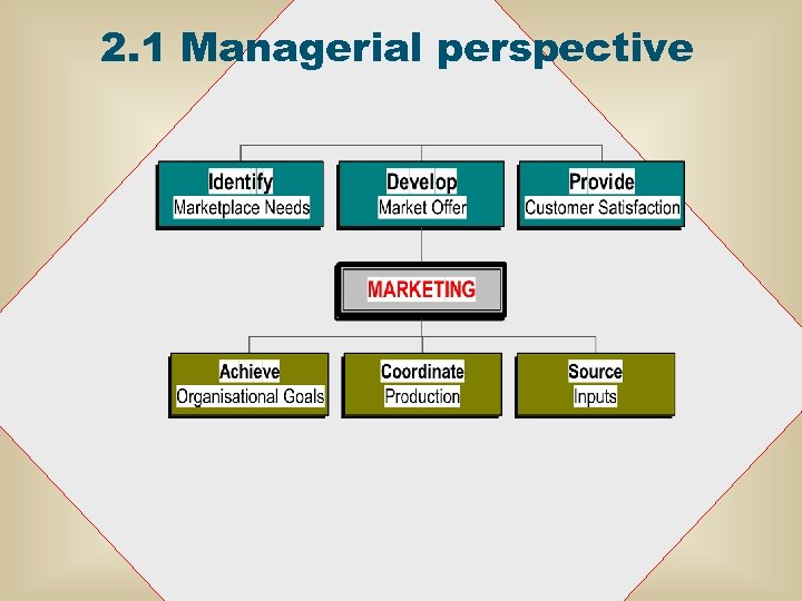2. 1 Managerial perspective

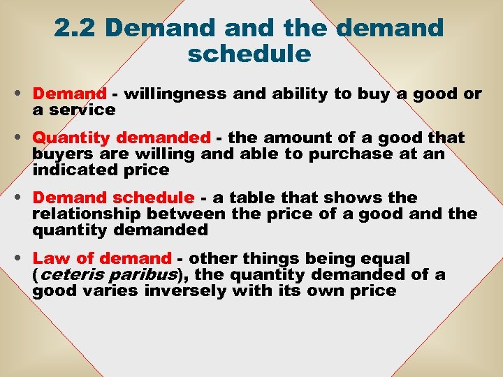2. 2 Demand the demand schedule • Demand - willingness and ability to buy a good or a service • Quantity demanded - the amount of a good that buyers are willing and able to purchase at an indicated price • Demand schedule - a table that shows the relationship between the price of a good and the quantity demanded • Law of demand - other things being equal (ceteris paribus), the quantity demanded of a good varies inversely with its own price

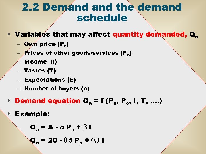2. 2 Demand the demand schedule • Variables that may affect quantity demanded, Qa – Own price (Pa) – Prices of other goods/services (Po) – Income (I) – Tastes (T) – Expectations (E) – Number of buyers (n) • Demand equation Qa = f (Pa, Po, I, T, …. ) • Example: Q a = A - a Pa + b I Qa = 20 - 0. 5 Pa + 0. 3 I

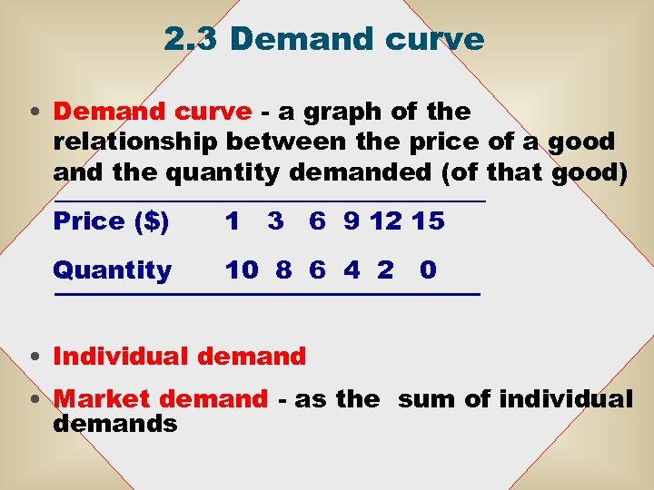2. 3 Demand curve • Demand curve - a graph of the relationship between the price of a good and the quantity demanded (of that good) Price ($) 1 3 6 9 12 15 Quantity 10 8 6 4 2 0 • Individual demand • Market demand - as the sum of individual demands

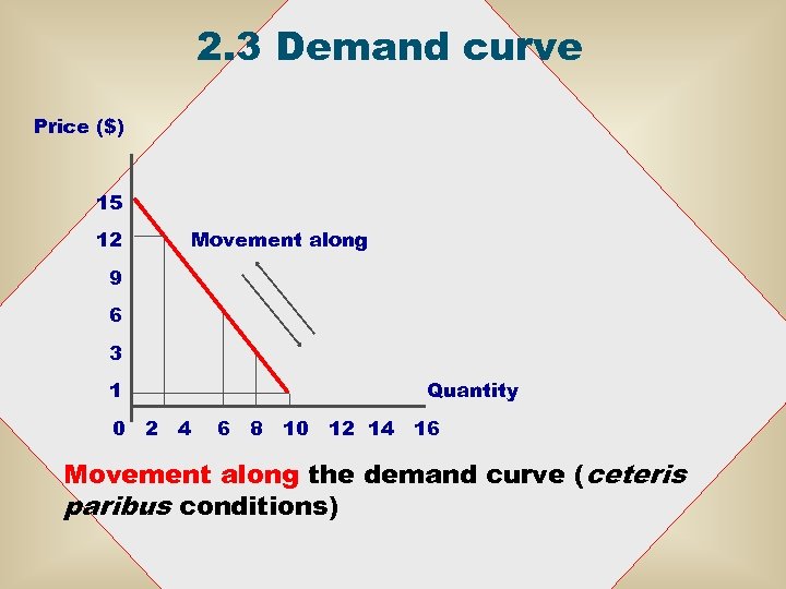2. 3 Demand curve Price ($) 15 12 Movement along 9 6 3 1 0 2 4 Quantity 6 8 10 12 14 16 Movement along the demand curve (ceteris paribus conditions)

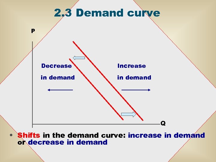2. 3 Demand curve P Decrease Increase in demand Q • Shifts in the demand curve: increase in demand or decrease in demand

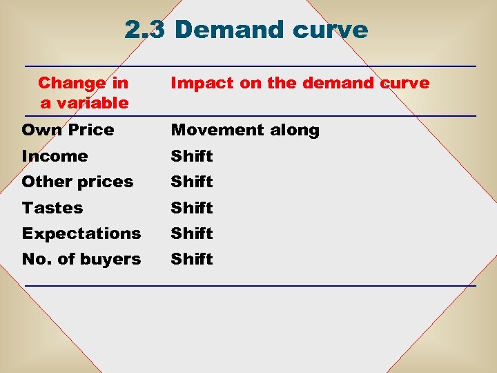2. 3 Demand curve Change in a variable Impact on the demand curve Own Price Movement along Income Shift Other prices Shift Tastes Shift Expectations Shift No. of buyers Shift

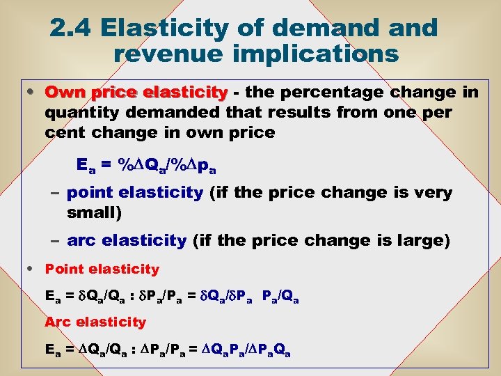2. 4 Elasticity of demand revenue implications • Own price elasticity - the percentage change in quantity demanded that results from one per cent change in own price Ea = %DQa/%Dpa – point elasticity (if the price change is very small) – arc elasticity (if the price change is large) • Point elasticity Ea = d. Qa/Qa : d. Pa/Pa = d. Qa/d. Pa Pa/Qa Arc elasticity Ea = DQa/Qa : DPa/Pa = DQa. Pa/DPa. Qa

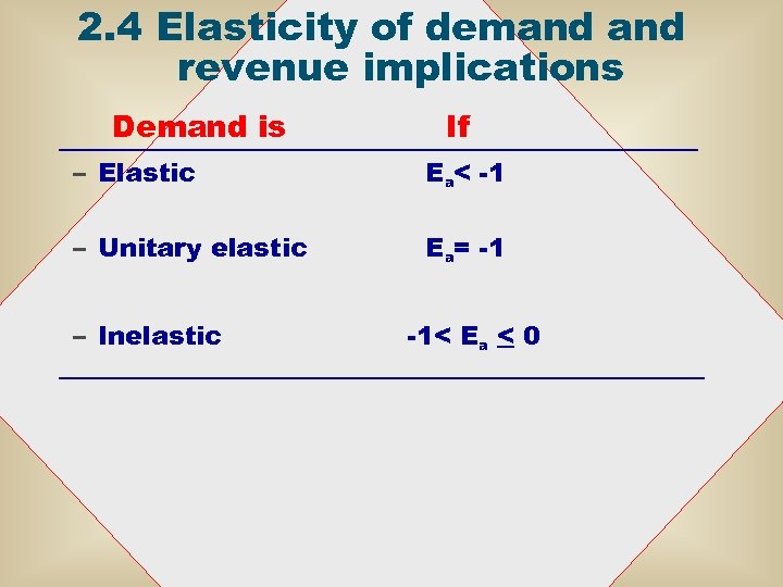2. 4 Elasticity of demand revenue implications Demand is If – Elastic Ea< -1 – Unitary elastic Ea= -1 – Inelastic -1< Ea < 0

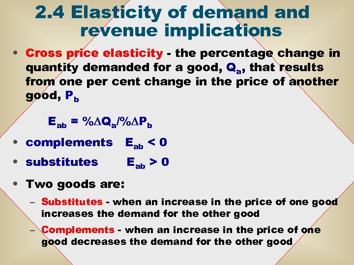2. 4 Elasticity of demand revenue implications • Cross price elasticity - the percentage change in quantity demanded for a good, Qa, that results from one per cent change in the price of another good, Pb Eab = %DQa/%DPb • complements Eab < 0 • substitutes Eab > 0 • Two goods are: – Substitutes - when an increase in the price of one good increases the demand for the other good – Complements - when an increase in the price of one good decreases the demand for the other good

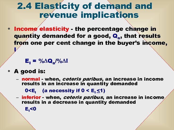2. 4 Elasticity of demand revenue implications • Income elasticity - the percentage change in quantity demanded for a good, Qa, that results from one per cent change in the buyer’s income, I EI = %DQa/%DI • A good is: – normal - when, ceteris paribus, an increase in income results in an increase in quantity demanded 0

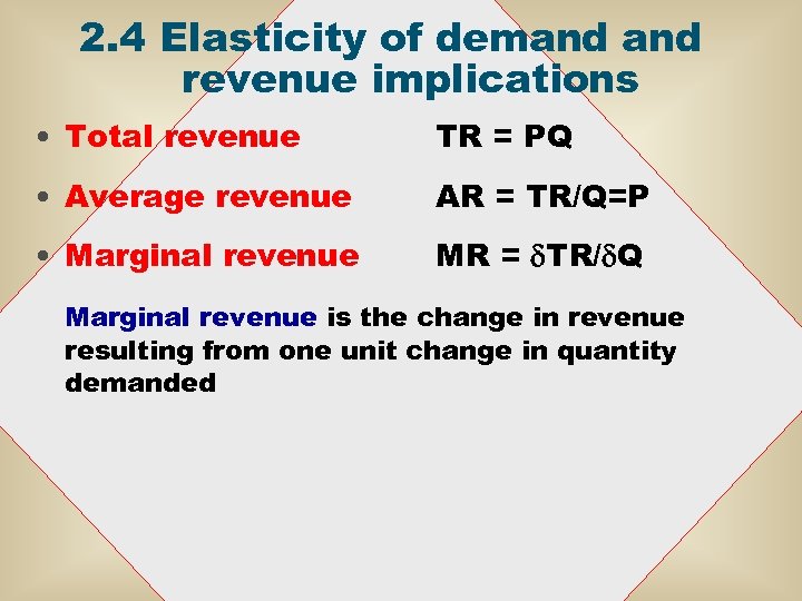2. 4 Elasticity of demand revenue implications • Total revenue TR = PQ • Average revenue AR = TR/Q=P • Marginal revenue MR = d. TR/d. Q Marginal revenue is the change in revenue resulting from one unit change in quantity demanded

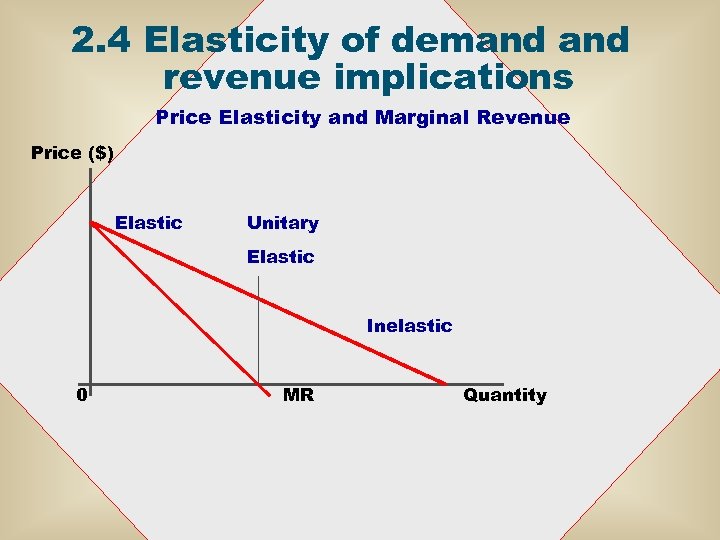2. 4 Elasticity of demand revenue implications Price Elasticity and Marginal Revenue Price ($) Elastic Unitary Elastic Inelastic 0 MR Quantity

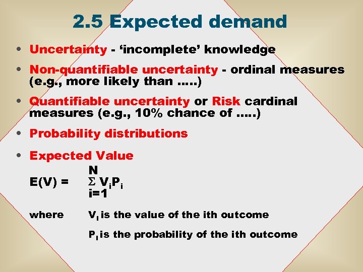2. 5 Expected demand • Uncertainty - ‘incomplete’ knowledge • Non-quantifiable uncertainty - ordinal measures (e. g. , more likely than …. . ) • Quantifiable uncertainty or Risk cardinal measures (e. g. , 10% chance of. …. ) • Probability distributions • Expected Value N E(V) = S V i. P i i=1 where Vi is the value of the ith outcome Pi is the probability of the ith outcome

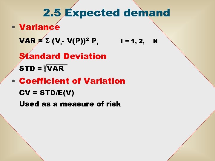2. 5 Expected demand • Variance VAR = S (Vi- V(P))2 Pi i = 1, 2, Standard Deviation STD = VAR • Coefficient of Variation CV = STD/E(V) Used as a measure of risk N

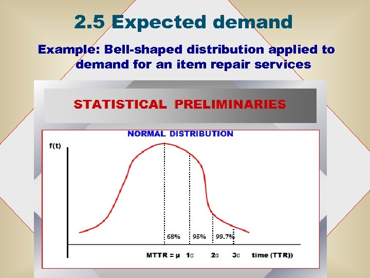2. 5 Expected demand Example: Bell-shaped distribution applied to demand for an item repair services

2. 5 Expected demand • Preferences for risk bearing – risk neutrality – risk preference – risk aversion – certainty equivalence – risk premium • Consider two gifts with equal E(V) but different coefficients of variation, CV. For example, Gift A - $100 cash Gift B - a lottery ticket offering a 50 -50 chance of winning $200 or nothing

2. 5 Expected demand • Risk-neutral person is indifferent between A and B • Risk-averse person prefers A to B • Risk-loving person prefers B to A • Certainty equivalent is a certain activity with E(V) equal to E(V) of some equivalent risky activity (e. g. , A is the certainty equivalent of B) • Risk premium is the difference between the subjective value of a risky activity and the value of its certainty equivalent (e. g. , V(B) - V(A))

2. 6 Further reading Baye (2010): chs. 3 -4