When is Too Much Inequality Not Enough The

When is “Too Much” Inequality Not Enough? The Selection of Israeli Emigrants Eric D. Gould Hebrew University Omer Moav Royal Holloway and Hebrew University 1

(Only) Two Things Israelis Agree Upon • There is “too much” inequality in Israel. • Israel suffers from a “Brain Drain. ” 2

“Too Much” Inequality in Israel • Israel Social Security Agency • Every 6 months: “poverty report” • Brandolini and Smeeding (2008) • Among 24 high income countries, only the US has a higher 90 -10 ratio in disposable personal income. 3

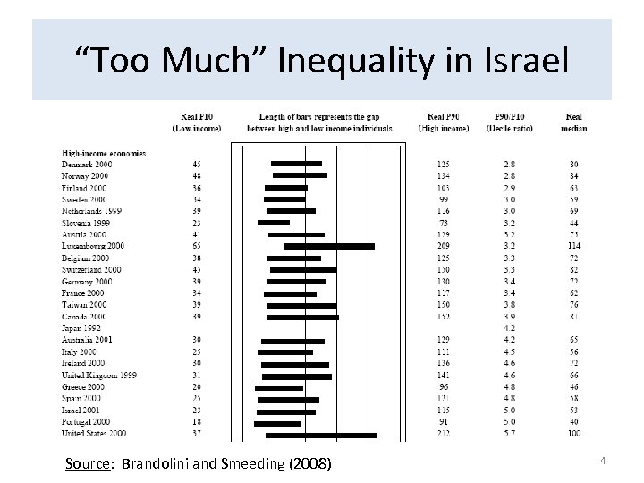“Too Much” Inequality in Israel Source: Brandolini and Smeeding (2008) 4

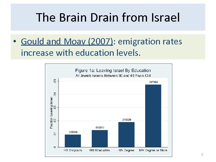The Brain Drain from Israel • Gould and Moav (2007): emigration rates increase with education levels. 5

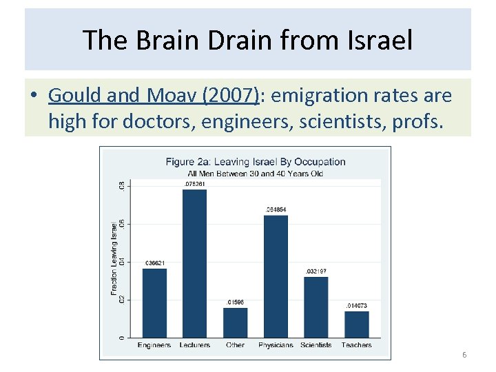The Brain Drain from Israel • Gould and Moav (2007): emigration rates are high for doctors, engineers, scientists, profs. 6

The Brain Drain from Israel • Dan Ben-David (2008) looks at academics. • The number of Israelis in the top 40 American departments in physics, chemistry, philosophy, computer science and economics, as a percentage of their remaining colleagues in Israel, is over twice the overall academic emigration rates from European countries. 7

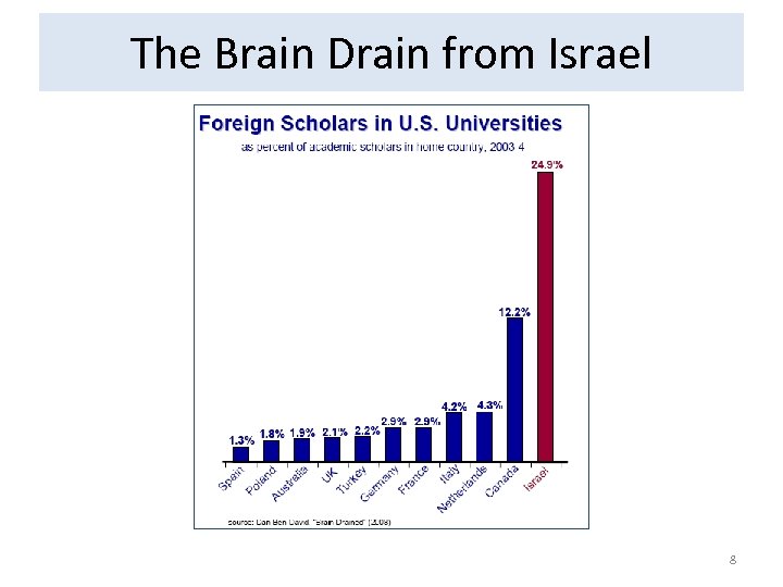The Brain Drain from Israel 8

(Only) Two Things Israelis Agree Upon • There is “too much” inequality in Israel. • Israel suffers from a “Brain Drain. ” • Our paper: solving one of these problems, may make the other one worse. • Main idea: A “Brain Drain” may be indicative of “too little” inequality. (Borjas (1987), Roy (1951)) 9

Goals of the Paper • Examine the effect of inequality on the incentives to emigrate according to skill levels. • Theoretically and empirically. • For Two types of skills: observable (education) and unobservable (residual wages) 10

Unique Data • 1995 Israeli Census • Matched with info on who leaves the country during the next 9 years. • Unique: wages of those who stay and leave. • Existing Literature: rare to have wage info on emigrants before they leave (the home country). 11

Unique Data • Existing Literature: rare to have wage info on emigrants before they leave (the home country). • Without wages: cannot assess selection based on wages, unobservable skill, etc. • Existing Literature: examines mostly education • But, education explains little variation in earnings. 12

Main Contributions • Empirical: analysis of emigrant selection based on observable and unobservable skill. • Theoretical: incorporate the notion of countryspecific skills into the analysis. 13

Outline of the Talk • Present the Borjas model and discuss the evidence. • Present the basic patterns of the data. • Show that the basic predictions work for observable skills but not for unobservable skills. • Present a model which explains why this is so. • Empirical Work. 14

Borjas (1987) Model of Emigration • Based on Roy (1951) model. • A person maximizes wages. • Wage in “Home” country: w 0 = α 0+β 0 skill • Wage in “Host” country: w 1 = α 1+β 1 skill • A person decides to emigrate if: w 1 > w 0 15

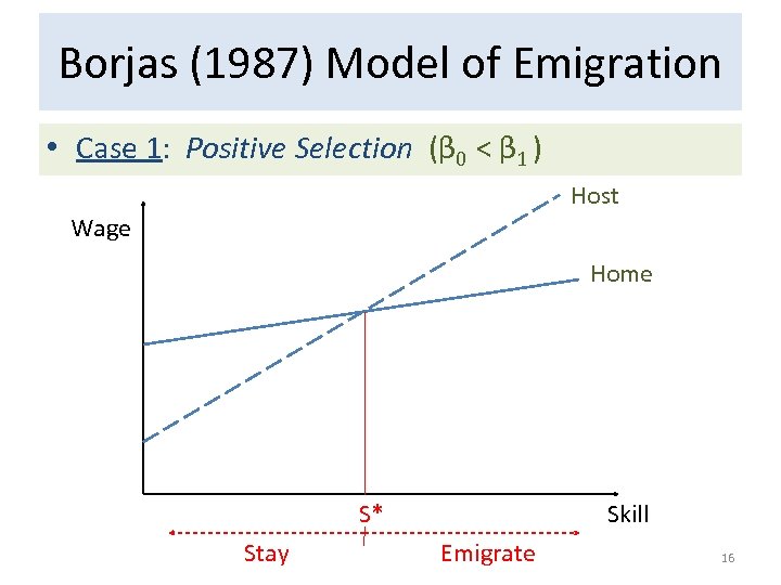Borjas (1987) Model of Emigration • Case 1: Positive Selection (β 0 < β 1 ) Host Wage Home S* Stay Skill Emigrate 16

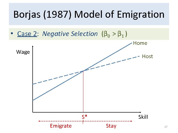Borjas (1987) Model of Emigration • Case 2: Negative Selection (β 0 > β 1 ) Home Wage Host S* Emigrate Skill Stay 17

Borjas (1987) Model of Emigration • Inequality affects the selection of immigrants. • Low inequality (β 0 < β 1 ) induces a Brain Drain. • This is true even if β 0 is considered “high. ” • Relative Inequality is what matters. 18

Evidence on the Borjas (1987) Model • Some evidence using immigrant wages from different countries in the US. – (Borjas (1987), Cobb-Clark (1993)) • Selection by education in US or OECD: very mixed – (Feliciano (2005), Grogger and Hanson (2008), Belot and Hatton (2008)). • Possible explanation: comparisons across countries may be confounded by other differences across countries (different moving costs, language, etc). 19

Evidence on the Borjas (1987) Model • Large Literature on the selection of Mexican immigrants in the US according to education. • Borjas model predicts negative selection – since the returns to education are higher in Mexico. • Chiquiar and Hanson (JPE, 2005) find “intermediate selection, ” not negative selection. 20

Chiquiar and Hanson (JPE, 2005) • Find “intermediate”, not negative selection. • They add “moving costs” to the model which decline with education levels. • Chiswick (1999) and Mc. Kenzie and Rapoport (2007) also argue that migration costs decline with education. 21

Chiquiar and Hanson (JPE, 2005) • Find “intermediate”, not negative selection. • Low education → low emigration due to high moving costs. • High education → low emigration due to high return to education in Mexico. • Mid-level education → highest rate of emigration. 22

Chiquiar and Hanson (JPE, 2005) • They look only at selection in terms of education. • We also find “intermediate selection” for wages. • Their explanation cannot be used to explain this. – Since returns to skill are higher in US versus Israel. • Therefore, we add “country-specific” skills to model. 23

Data • 1995 Israeli Census – contains demographic, labor force, information • Merged with an indicator for being a “mover” as of 2002 and 2004. – if he is a “mover, ” we also have the year he moved. • “Mover” = out of Israel more than a year. 24

Weaknesses in the Data • No info on where he “moved. ” (most are in US) • No info on whether he intends to come back. – All papers on emigration suffer from this. – The individual probably does not know this. • Our strategy: check robustness of results to different ways of defining a “mover. ” 25

Strengths in the Data • Info on everyone before they decide to move. • Wages, education, occupation, industry, etc. • We can see where they are in the distribution of observable skill (education) and unobservable skill (wages) before they leave. 26

Our Sample • A strong attachment to the labor force. – at least 30 hrs a week, 6 months in previous year – not self-employed. • Males • ≥ 30 years old as of 1995 (finished schooling) • Young enough so that the moving decision is likely to be career related. (30 -45 years old in 1995) 27

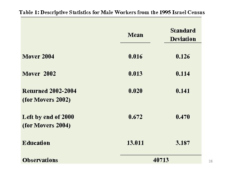Table 1: Descriptive Statistics for Male Workers from the 1995 Israel Census Mean Standard Deviation Mover 2004 0. 016 0. 126 Mover 2002 0. 013 0. 114 Returned 2002 -2004 (for Movers 2002) 0. 020 0. 141 Left by end of 2000 (for Movers 2004) 0. 672 0. 470 Education 13. 011 3. 187 Observations 40713 28

Emigration increases with education 29

Levels are higher for Non-Natives 30

Pattern is Similar for Earlier Ages 31

Pattern is Similar for Earlier Ages 32

No Selection on Returning Israelis 33

Emigration and Residual Wages: Inverse U-Shape 34

Emigration and Residual Wages: Inverse U-Shape 35

Emigration and Residual Wages: Inverse U-Shape 36

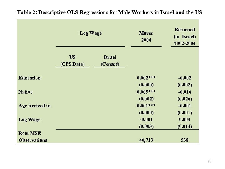Table 2: Descriptive OLS Regressions for Male Workers in Israel and the US Log Wage US (CPS Data) Education Native Age Arrived in Log Wage Root MSE Observations Mover 2004 Returned (to Israel) 2002 -2004 0. 002*** (0. 000) 0. 005*** (0. 002) 0. 001*** (0. 000) -0. 001 (0. 003) -0. 002 (0. 002) -0. 016 (0. 026) -0. 001 (0. 001) 0. 003 (0. 014) 40, 713 538 Israel (Census) 37

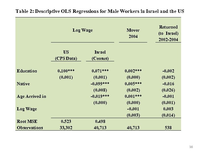Table 2: Descriptive OLS Regressions for Male Workers in Israel and the US Mover 2004 Log Wage US (CPS Data) Education 0. 071*** (0. 001) -0. 099*** (0. 008) -0. 019*** (0. 000) 0. 523 33, 302 0. 498 40, 713 Native Age Arrived in Log Wage Root MSE Observations 0. 002*** (0. 000) 0. 005*** (0. 002) 0. 001*** (0. 000) -0. 001 (0. 003) -0. 002 (0. 002) -0. 016 (0. 026) -0. 001 (0. 001) 0. 003 (0. 014) 40, 713 538 Israel (Census) 0. 100*** (0. 001) Returned (to Israel) 2002 -2004 38

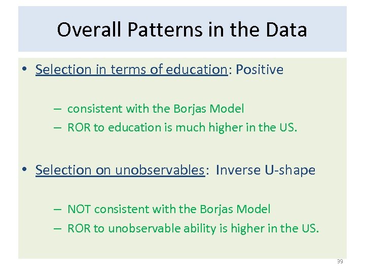Overall Patterns in the Data • Selection in terms of education: Positive – consistent with the Borjas Model – ROR to education is much higher in the US. • Selection on unobservables: Inverse U-shape – NOT consistent with the Borjas Model – ROR to unobservable ability is higher in the US. 39

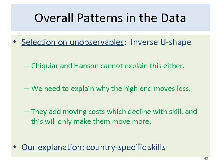Overall Patterns in the Data • Selection on unobservables: Inverse U-shape – Chiquiar and Hanson cannot explain this either. – We need to explain why the high end moves less. – They add moving costs which decline with skill, and this will only make them move more. • Our explanation: country-specific skills 40

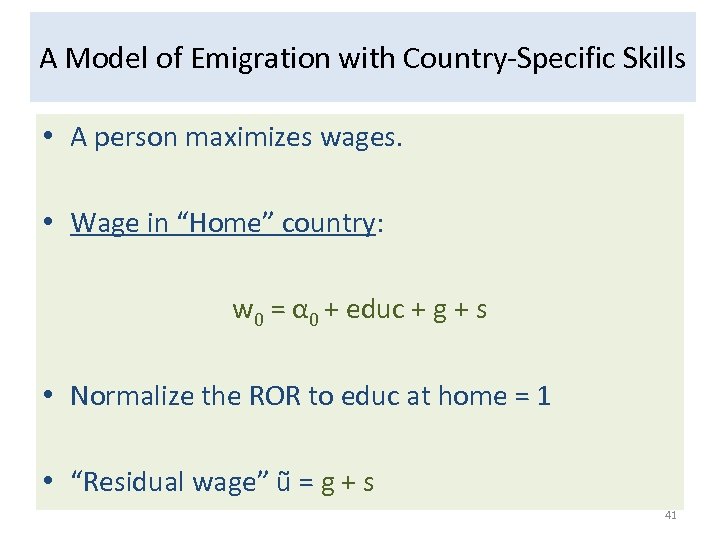A Model of Emigration with Country-Specific Skills • A person maximizes wages. • Wage in “Home” country: w 0 = α 0 + educ + g + s • Normalize the ROR to educ at home = 1 • “Residual wage” ũ = g + s 41

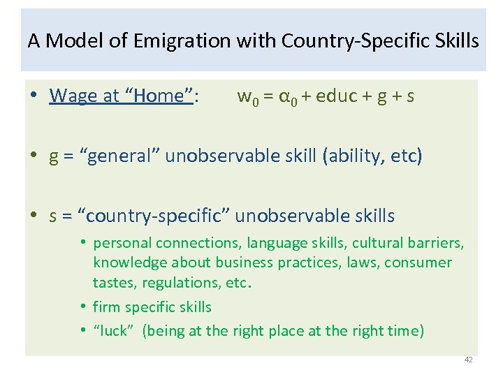A Model of Emigration with Country-Specific Skills • Wage at “Home”: w 0 = α 0 + educ + g + s • g = “general” unobservable skill (ability, etc) • s = “country-specific” unobservable skills • personal connections, language skills, cultural barriers, knowledge about business practices, laws, consumer tastes, regulations, etc. • firm specific skills • “luck” (being at the right place at the right time) 42

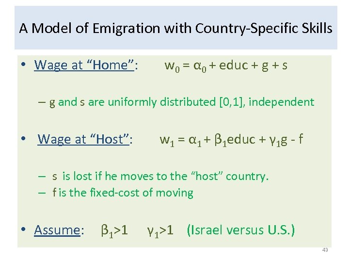A Model of Emigration with Country-Specific Skills • Wage at “Home”: w 0 = α 0 + educ + g + s – g and s are uniformly distributed [0, 1], independent • Wage at “Host”: w 1 = α 1 + β 1 educ + γ 1 g - f – s is lost if he moves to the “host” country. – f is the fixed-cost of moving • Assume: β 1>1 γ 1>1 (Israel versus U. S. ) 43

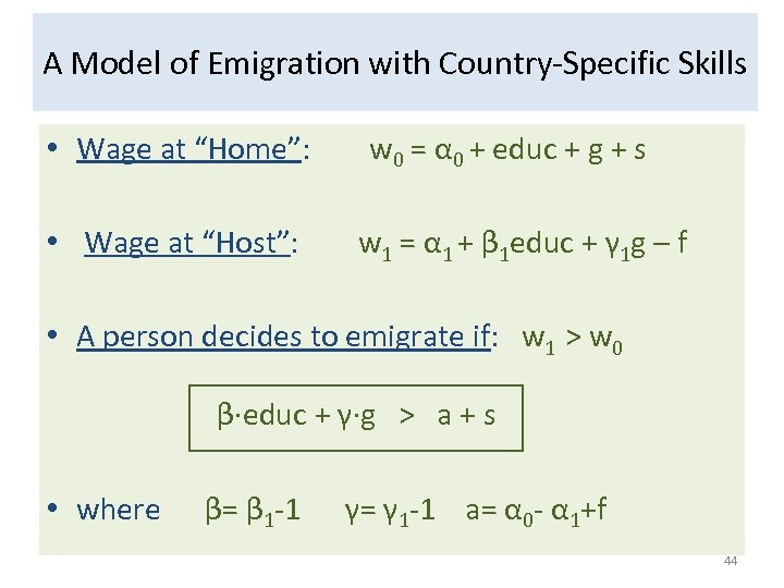A Model of Emigration with Country-Specific Skills • Wage at “Home”: • Wage at “Host”: w 0 = α 0 + educ + g + s w 1 = α 1 + β 1 educ + γ 1 g – f • A person decides to emigrate if: w 1 > w 0 β∙educ + γ∙g > a + s • where β= β 1 -1 γ= γ 1 -1 a= α 0 - α 1+f 44

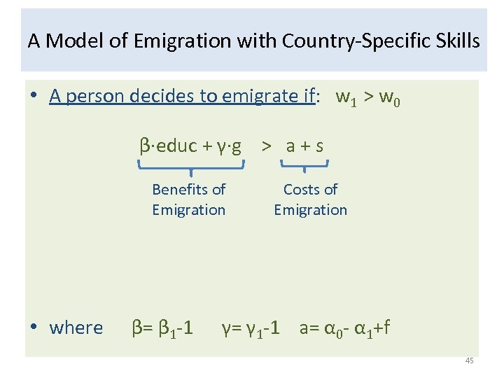A Model of Emigration with Country-Specific Skills • A person decides to emigrate if: w 1 > w 0 β∙educ + γ∙g > a + s Benefits of Emigration • where β= β 1 -1 Costs of Emigration γ= γ 1 -1 a= α 0 - α 1+f 45

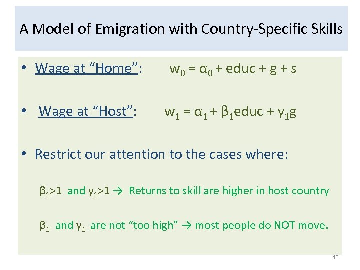A Model of Emigration with Country-Specific Skills • Wage at “Home”: w 0 = α 0 + educ + g + s • Wage at “Host”: w 1 = α 1 + β 1 educ + γ 1 g • Restrict our attention to the cases where: β 1>1 and γ 1>1 → Returns to skill are higher in host country β 1 and γ 1 are not “too high” → most people do NOT move. 46

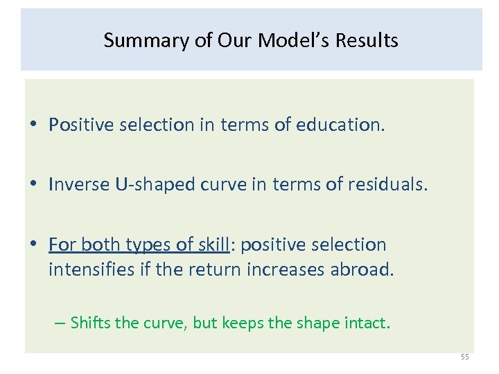
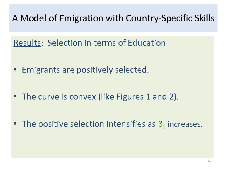A Model of Emigration with Country-Specific Skills Results: Selection in terms of Education • Emigrants are positively selected. • The curve is convex (like Figures 1 and 2). • The positive selection intensifies as β 1 increases. 47

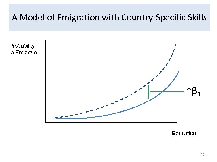A Model of Emigration with Country-Specific Skills Probability to Emigrate ↑β 1 Education 48

Positive and Convex Selection 49

A Model of Emigration with Country-Specific Skills Results: Selection in terms of Residual Wage = g + s • Inverse U-shaped function (like Figures 4 -6) • The positive selection intensifies as γ 1 increases. – The curves shifts right, but u-shape remains intact. 50

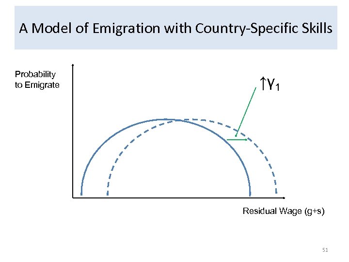A Model of Emigration with Country-Specific Skills Probability to Emigrate ↑γ 1 Residual Wage (g+s) 51

Emigration and Residual Wages: Inverse U-Shape 52

A Model of Emigration with Country-Specific Skills • Intuition: Inverse U-shaped function • A person emigrates if: β∙educ + γ∙g > a + s Benefits of Emigration Costs of Emigration • Person’s Residual = g + s • g increases the probability of emigrating • s decreases the probability of emigrating • Therefore, a higher g/s increases the chances to emigrate. 53

A Model of Emigration with Country-Specific Skills • Who is more likely to have a high g/s ratio? • High residual wage → g and s are high, so g/s ≈ 1 • Low residual wage → g and s are low, so g/s ≈ 1 • Mid-level residuals → variation in g and s, g/s varies – If g/s is high, more likely that you are in the middle of the residual wage distribution than in the tails. 54

Summary of Our Model’s Results • Positive selection in terms of education. • Inverse U-shaped curve in terms of residuals. • For both types of skill: positive selection intensifies if the return increases abroad. – Shifts the curve, but keeps the shape intact. 55

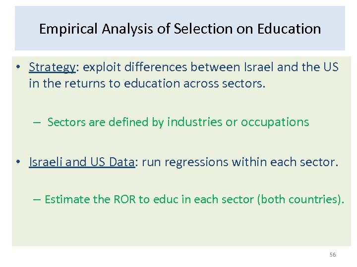Empirical Analysis of Selection on Education • Strategy: exploit differences between Israel and the US in the returns to education across sectors. – Sectors are defined by industries or occupations • Israeli and US Data: run regressions within each sector. – Estimate the ROR to educ in each sector (both countries). 56

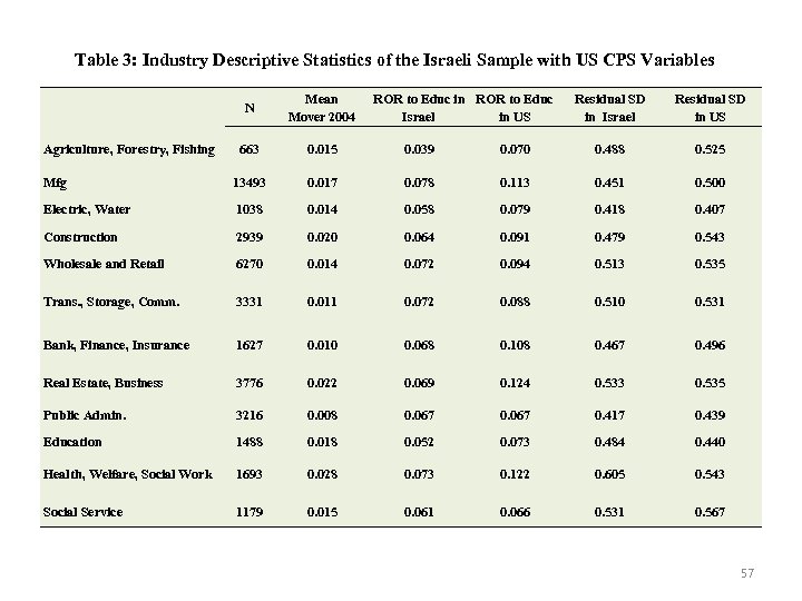Table 3: Industry Descriptive Statistics of the Israeli Sample with US CPS Variables N Mean Mover 2004 Residual SD in Israel Residual SD in US 663 0. 015 0. 039 0. 070 0. 488 0. 525 Mfg 13493 0. 017 0. 078 0. 113 0. 451 0. 500 Electric, Water 1038 0. 014 0. 058 0. 079 0. 418 0. 407 Construction 2939 0. 020 0. 064 0. 091 0. 479 0. 543 Wholesale and Retail 6270 0. 014 0. 072 0. 094 0. 513 0. 535 Trans. , Storage, Comm. 3331 0. 011 0. 072 0. 088 0. 510 0. 531 Bank, Finance, Insurance 1627 0. 010 0. 068 0. 108 0. 467 0. 496 Real Estate, Business 3776 0. 022 0. 069 0. 124 0. 533 0. 535 Public Admin. 3216 0. 008 0. 067 0. 417 0. 439 Education 1488 0. 018 0. 052 0. 073 0. 484 0. 440 Health, Welfare, Social Work 1693 0. 028 0. 073 0. 122 0. 605 0. 543 Social Service 1179 0. 015 0. 061 0. 066 0. 531 0. 567 Agriculture, Forestry, Fishing ROR to Educ in ROR to Educ Israel in US 57

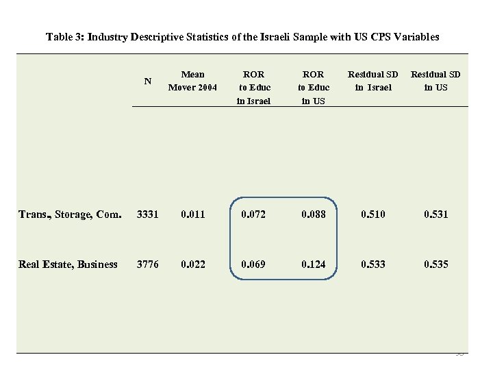Table 3: Industry Descriptive Statistics of the Israeli Sample with US CPS Variables N Mean Mover 2004 ROR to Educ in Israel ROR to Educ in US Residual SD in Israel Residual SD in US Trans. , Storage, Com. 3331 0. 011 0. 072 0. 088 0. 510 0. 531 Real Estate, Business 3776 0. 022 0. 069 0. 124 0. 533 0. 535 58

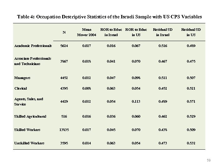Table 4: Occupation Descriptive Statistics of the Israeli Sample with US CPS Variables N Mean Mover 2004 ROR to Educ in Israel in US Residual SD in Israel Residual SD in US Academic Professionals 5624 0. 027 0. 016 0. 067 0. 516 0. 489 Associate Professionals and Technicians 3867 0. 018 0. 041 0. 070 0. 467 0. 475 Managers 4452 0. 012 0. 047 0. 098 0. 511 0. 507 Clerical 4395 0. 008 0. 063 0. 054 0. 452 0. 521 Agents, Sales, and Service 4429 0. 012 0. 054 0. 113 0. 489 0. 571 Skilled Agricultural 516 0. 036 0. 060 0. 462 0. 529 Skilled Workers 13835 0. 017 0. 045 0. 070 0. 438 0. 509 Unskilled Workers 3595 0. 014 0. 063 0. 054 0. 473 0. 532 59

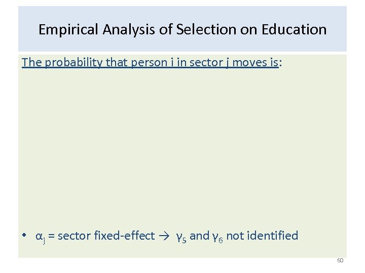Empirical Analysis of Selection on Education The probability that person i in sector j moves is: • αj = sector fixed-effect → γ 5 and γ 6 not identified 60

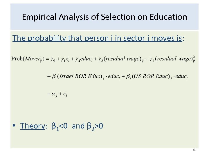Empirical Analysis of Selection on Education The probability that person i in sector j moves is: • Theory: β 1<0 and β 2>0 61

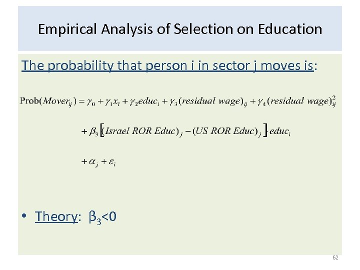Empirical Analysis of Selection on Education The probability that person i in sector j moves is: • Theory: β 3<0 62

Comments on the Empirical Strategy • We do not assume that everyone moves to the US • Although most of them do. • 123, 000 in US (Global Migrant Origin Database) • Next highest (non-Muslim country) is Canada: 17, 000 • We do not assume that individuals do not change sectors. • We are checking to see if these factors are important. 63

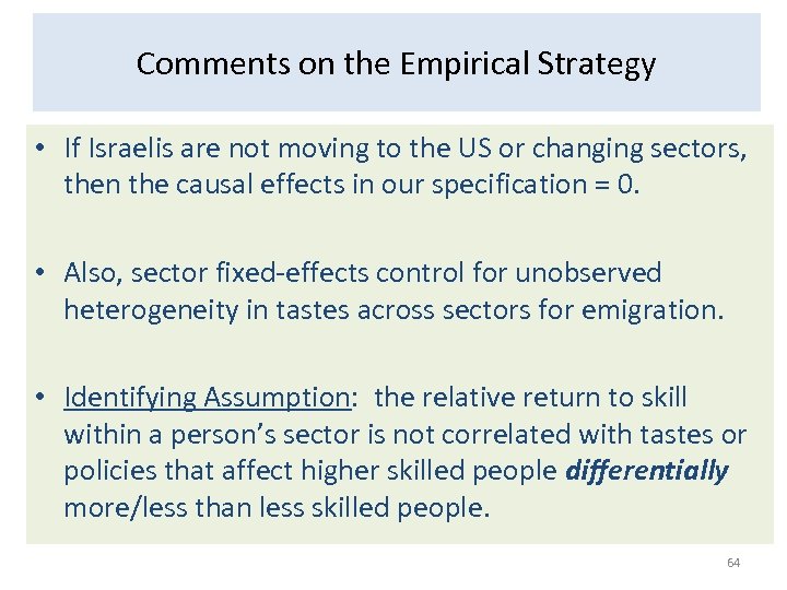Comments on the Empirical Strategy • If Israelis are not moving to the US or changing sectors, then the causal effects in our specification = 0. • Also, sector fixed-effects control for unobserved heterogeneity in tastes across sectors for emigration. • Identifying Assumption: the relative return to skill within a person’s sector is not correlated with tastes or policies that affect higher skilled people differentially more/less than less skilled people. 64

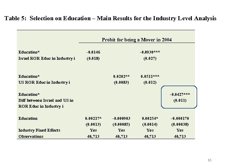Table 5: Selection on Education – Main Results for the Industry Level Analysis Probit for being a Mover in 2004 Education* Israel ROR Educ in Industry i -0. 0146 (0. 018) Education* US ROR Educ in Industry i -0. 0930*** (0. 027) 0. 0202** (0. 0083) 0. 0511*** (0. 012) Education* Diff between Israel and US in ROR Educ in Industry i Education Industry Fixed Effects Observations -0. 0427*** (0. 011) 0. 00217* (0. 0013) Yes 40, 713 -0. 000903 (0. 00085) Yes 40, 713 0. 00254* (0. 0014) Yes 40, 713 -0. 000170 (0. 00038) Yes 40, 713 65

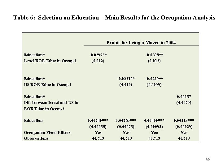Table 6: Selection on Education – Main Results for the Occupation Analysis Probit for being a Mover in 2004 Education* Israel ROR Educ in Occup i -0. 0297** (0. 012) Education* US ROR Educ in Occup i -0. 0298** (0. 012) -0. 0221** (0. 010) -0. 0219** (0. 0099) Education* Diff between Israel and US in ROR Educ in Occup i Education Occupation Fixed Effects Observations 0. 00157 (0. 0079) 0. 00240*** (0. 00058) Yes 40, 713 0. 00269*** (0. 00075) Yes 40, 713 0. 00400*** (0. 00093) Yes 40, 713 0. 00113*** (0. 00029) Yes 40, 713 66

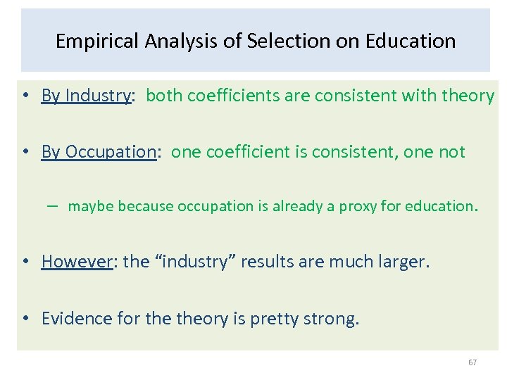Empirical Analysis of Selection on Education • By Industry: both coefficients are consistent with theory • By Occupation: one coefficient is consistent, one not – maybe because occupation is already a proxy for education. • However: the “industry” results are much larger. • Evidence for theory is pretty strong. 67

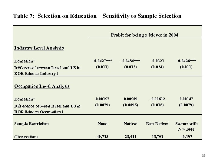Table 7: Selection on Education – Sensitivity to Sample Selection Probit for being a Mover in 2004 Industry Level Analysis -0. 0427*** (0. 011) -0. 0484*** (0. 012) -0. 0321 (0. 024) -0. 0426*** (0. 011) 0. 00157 (0. 0079) 0. 00509 (0. 0096) -0. 00612 (0. 016) 0. 00147 (0. 0079) Sample Restriction None Natives Non-Natives Sectors with N > 1000 Observations 40, 713 25, 011 15, 702 40, 197 Education* Diff erence between Israel and US in ROR Educ in Industry i Occupation Level Analysis Education* Diff erence between Israel and US in ROR Educ in Occupation i 68

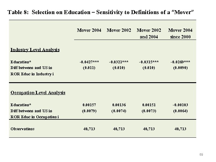Table 8: Selection on Education – Sensitivity to Definitions of a “Mover” Mover 2004 Mover 2002 and 2004 Mover 2004 since 2000 -0. 0427*** (0. 011) -0. 0321*** (0. 010) -0. 0315*** (0. 010) -0. 0269*** (0. 0090) 0. 00157 (0. 0079) 0. 00136 (0. 0074) 0. 00151 (0. 0073) -0. 00103 (0. 0064) 40, 713 Industry Level Analysis Education* Diff between and US in ROR Educ in Industry i Occupation Level Analysis Education* Diff between and US in ROR Educ in Occupation i Observations 69

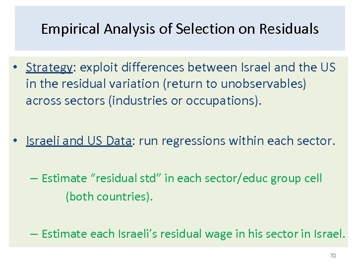Empirical Analysis of Selection on Residuals • Strategy: exploit differences between Israel and the US in the residual variation (return to unobservables) across sectors (industries or occupations). • Israeli and US Data: run regressions within each sector. – Estimate “residual std” in each sector/educ group cell (both countries). – Estimate each Israeli’s residual wage in his sector in Israel. 70

Empirical Analysis of Selection on Residuals Prob that person i in sector j and educ group k moves is: • αjk = cell fixed-effect 71

Empirical Analysis of Selection on Residuals Prob that person i in sector j and educ group k moves is: • Theory: β 1<0 and β 2>0 72

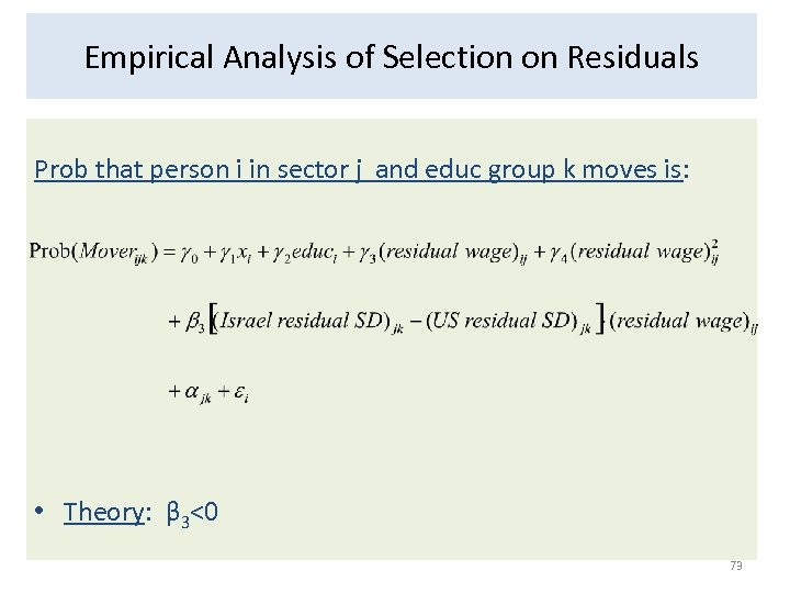Empirical Analysis of Selection on Residuals Prob that person i in sector j and educ group k moves is: • Theory: β 3<0 73

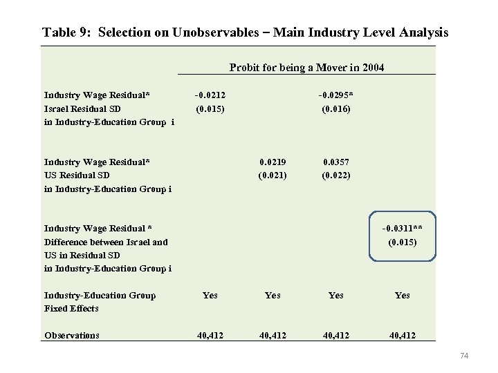Table 9: Selection on Unobservables – Main Industry Level Analysis Probit for being a Mover in 2004 Industry Wage Residual* Israel Residual SD in Industry-Education Group i -0. 0212 (0. 015) Industry Wage Residual* US Residual SD in Industry-Education Group i -0. 0295* (0. 016) 0. 0219 (0. 021) 0. 0357 (0. 022) Industry Wage Residual * Difference between Israel and US in Residual SD in Industry-Education Group i Industry-Education Group Fixed Effects Observations -0. 0311** (0. 015) Yes Yes 40, 412 74

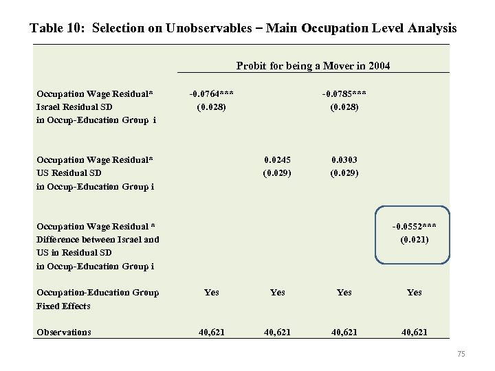Table 10: Selection on Unobservables – Main Occupation Level Analysis Probit for being a Mover in 2004 Occupation Wage Residual* Israel Residual SD in Occup-Education Group i -0. 0764*** (0. 028) Occupation Wage Residual* US Residual SD in Occup-Education Group i -0. 0785*** (0. 028) 0. 0245 (0. 029) 0. 0303 (0. 029) Occupation Wage Residual * Difference between Israel and US in Residual SD in Occup-Education Group i Occupation-Education Group Fixed Effects Observations -0. 0552*** (0. 021) Yes Yes 40, 621 75

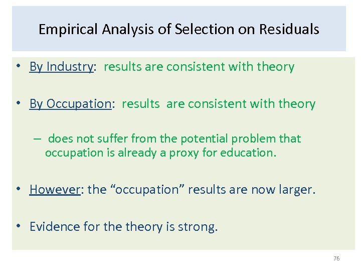Empirical Analysis of Selection on Residuals • By Industry: results are consistent with theory • By Occupation: results are consistent with theory – does not suffer from the potential problem that occupation is already a proxy for education. • However: the “occupation” results are now larger. • Evidence for theory is strong. 76

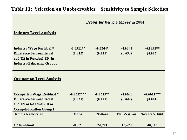Table 11: Selection on Unobservables – Sensitivity to Sample Selection Probit for being a Mover in 2004 Industry Level Analysis Industry Wage Residual * Difference between Israel and US in Residual SD in Industry-Education Group i -0. 0311** (0. 015) -0. 0244* (0. 014) -0. 0340 (0. 033) -0. 0331** (0. 015) -0. 0552*** (0. 021) -0. 0515** (0. 023) -0. 0636 (0. 044) -0. 0621*** (0. 021) None Natives Non-Natives Sectors > 1000 40, 621 24, 573 15, 673 40, 105 Occupation Level Analysis Occupation Wage Residual * Difference between Israel and US in Residual SD in Occup-Education Group i Sample Restriction Observations 77

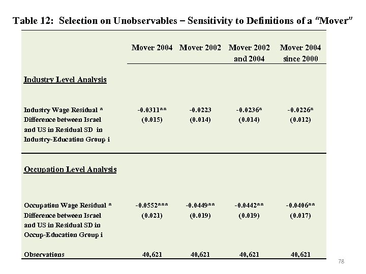Table 12: Selection on Unobservables – Sensitivity to Definitions of a “Mover” Mover 2004 Mover 2002 and 2004 Mover 2004 since 2000 Industry Level Analysis Industry Wage Residual * Difference between Israel and US in Residual SD in Industry-Education Group i -0. 0311** (0. 015) -0. 0223 (0. 014) -0. 0236* (0. 014) -0. 0226* (0. 012) -0. 0552*** (0. 021) -0. 0449** (0. 019) -0. 0442** (0. 019) -0. 0406** (0. 017) 40, 621 Occupation Level Analysis Occupation Wage Residual * Difference between Israel and US in Residual SD in Occup-Education Group i Observations 78

Further Robustness Checks in Tables 13 and 14 • Results are stronger using OLS instead of Probit • Results are robust to including interaction between residual squared and difference in residual variation. • Results are robust to using the residual rank (within each 5 -year age group) instead of residuals (since residual variation increases with age). • Results are robust to estimating selection on education and unobservables in one regression (Table 14). 79

Magnitude of the effects: Selection on Education 80

Magnitude of the effects: Selection on Education 81

Magnitude of the effects: Selection on Residuals 82

Magnitude of the effects: Selection on Residuals 83

Magnitude of the effects: Selection on Residuals 84

Magnitude of the effects: Selection on Residuals 85

Magnitude of the effects: Selection on Residuals 86

Conclusion • Analyzed selection on observable and unobservable skill. • Unique data (info on individuals before they move). • Added “country-specific” skills to the Borjas Model. • Theory is consistent with our results. – showing the importance of “country-specific” skills. • Results: Inequality does affect emigrant selection. 87

Conclusion • Results are unlikely due to policy by US immigration. • Policy cannot explain variation across sectors. • Strongest evidence in favor of the Borjas model. • Changes in inequality affect selection by shifting the curve. 88

Implications • Not all inequality is “bad. ” • High inequality in the US is perceived in a negative light. • But, this is how it attracts the best workers in the world. • A country’s level of inequality – determines how it will compete for its best workers. • Need to be careful about reducing inequality (by taxes) which will exacerbate the brain drain. 89