Welcome to Session 2 Graduate Workshop in Statistics

Welcome to Session 2 Graduate Workshop in Statistics Instructor: Kam Hamidieh Monday July 18, 2005

Today’s Agenda • Any Questions? • Brief Review from last time • Main topics today – Finish up descriptive statistics – Crash course in Probability • Discussion of posted papers and Exercise Set 1 • Brief Demo of SPSS & R (if time permits) 2

Random Circumstances/Phenomena • A random circumstance or a random phenomenon is one in which the outcome is uncertain. • Examples: – Toss of a fair coin: heads or tails. – Toss of a fair (balanced) die: any number between 1 and 6 – Accuracy of a screening test: test shows positive when you don’t have the disease (false positives) – Weather status: sunny or rainy • Note: randomness ≠ chaos!!! 3

What is Probability? • A probability is a number between 0 and 1 that is assigned to a possible outcome of a random circumstance. • For the complete set of distinct possible outcomes of a random circumstance, the total of the assigned probabilities must equal 1. • Probability theory is the major tool in statistical inference. 4

Interpretations of Probabilities • Two major interpretations are: – Frequentist view: we define the probability of a random circumstance as the proportion of times it would occur over the long run. This is also sometimes called the relative frequency of a particular random circumstance. – Subjective or Personal probability: we define the probability of an event to be the degree to which a given individual believes the event will happen. 5

Determining Probabilities • Relative frequency probabilities can be determined by: – Making some assumptions about the physical world and using them to find relative frequencies – Observing the results of random circumstances over a long run – Measuring a representative sample and observing the relative frequencies of the sample that fall into various categories. • Data from similar events in the past and other knowledge are incorporated when determining personal probabilities. 6

Probability Models • We are interested in a random circumstance and we want to model it. • In the broadest sense, modeling means being able to assign probability values (between 0 and 1) to the possible outcomes of a random circumstance. • In the next few slides we’ll look at the constituents of probability models. 7

Probability Definitions and Terms • Sample space: the collection of unique, nonoverlapping possible outcomes of a random circumstance. • Simple event: one outcome in the sample space; a possible outcome of a random circumstance. • Event: a collection of one or more simple events in the sample space; often written as A, B, C, and so on. Technically it is some subset of the sample space. • It is often helpful to think of the occurrence of an event as the outcome of an experiment. 8

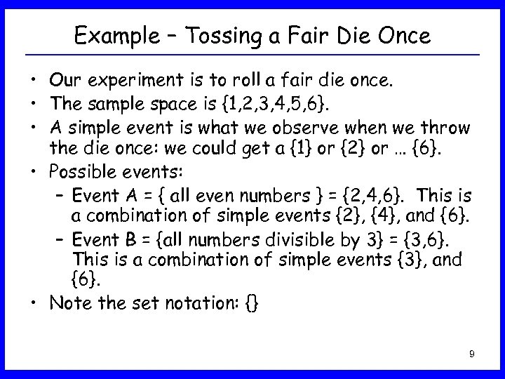Example – Tossing a Fair Die Once • Our experiment is to roll a fair die once. • The sample space is {1, 2, 3, 4, 5, 6}. • A simple event is what we observe when we throw the die once: we could get a {1} or {2} or … {6}. • Possible events: – Event A = { all even numbers } = {2, 4, 6}. This is a combination of simple events {2}, {4}, and {6}. – Event B = {all numbers divisible by 3} = {3, 6}. This is a combination of simple events {3}, and {6}. • Note the set notation: {} 9

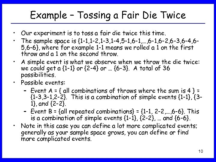Example – Tossing a Fair Die Twice • Our experiment is to toss a fair die twice this time. • The sample space is {1 -1, 1 -2, 1 -3, 1 -4, 5 -1, 6 -1, …, 6 -1, 6 -2, 6 -3, 6 -4, 65, 6 -6}, where for example 1 -1 means we rolled a 1 on the first throw and a 1 on the second throw. • A simple event is what we observe when we throw the die twice: we could get a {1 -1} or {2 -4} or … {6 -3}. A total of 36 possibilities. • Possible events: – Event A = { all combinations of throws where the sum is 4 } = {1 -3, 3 -1, 2 -2}. This is a combination of simple events {1 -1}, {31}, and {2 -2}. – Event B = {all repeated combinations} = {1 -1, 2 -2, …, 6 -6}. This is a combination of simple events {1 -1}, {2 -2}, … and {6 -6}. • Note in this case you can define a lot more complicated events; generally as your sample space grows, you can define or find more complicated events. 10

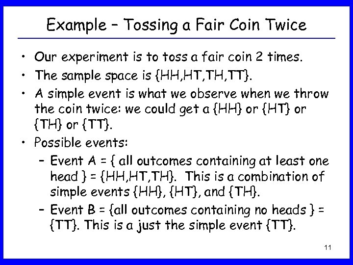Example – Tossing a Fair Coin Twice • Our experiment is to toss a fair coin 2 times. • The sample space is {HH, HT, TH, TT}. • A simple event is what we observe when we throw the coin twice: we could get a {HH} or {HT} or {TH} or {TT}. • Possible events: – Event A = { all outcomes containing at least one head } = {HH, HT, TH}. This is a combination of simple events {HH}, {HT}, and {TH}. – Event B = {all outcomes containing no heads } = {TT}. This is a just the simple event {TT}. 11

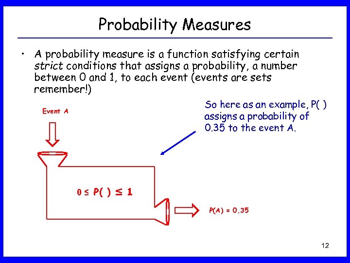Probability Measures • A probability measure is a function satisfying certain strict conditions that assigns a probability, a number between 0 and 1, to each event (events are sets remember!) So here as an example, P( ) assigns a probability of 0. 35 to the event A. Event A 0 ≤ P( ) ≤ 1 P(A) = 0. 35 12

Equally Likely Events • Equally Likely Simple Events: If there are k simple events in the sample space and they are all equally likely, then the probability of the occurrence of each one is 1/k. • All the following, have equally likely simple events: – Our experiment is to toss a fair die twice. The sample space is {1 -1, 1 -2, 1 -3, 1 -4, 5 -1, 6 -1, …, 6 -1, 6 -2, 6 -3, 6 -4, 6 -5, 66}. So then P({1 -1}) = P({1 -2}) = … = P({6 -6}) = 1/36. – Our experiment is to toss a fair die once. The sample space is {1, 2, 3, 4, 5, 6}. So then P({1}) = P({2}) = … = P({6}) = 1/6. – Our experiment is to flip a fair coin 2 times. The sample space is {HH, HT, TH, TT}. So P({HH}) = … = P({TT}) = ¼. 13

Complementary Events • One event is the complement of another event if the two events do not contain any of the same simple events and together they cover the entire sample space. • To emphasize, complementary events can not happen at the same time. 14

Example – Complementary Events • Our experiment is to toss a fair die once. The sample space is {1, 2, 3, 4, 5, 6}. • Possible complementary events are: – A = {1, 2, 3} and AC = {4, 5, 6} – B = {Odd outcome} = {1, 3, 5} and BC = {Even Outcome} = {2, 4, 6}. – F = {outcome divisible by 3} = {3, 6} and FC = {outcome not divisible by 3} = {1, 2, 4, 5}. • Note in all cases the event and its complement put together, give you the sample space. • Note also in all cases the event and its complement can not happen at the same time. 15

Mutually Exclusive Events • Two or more events are mutually exclusive if they do not contain any of the same simple events or outcomes. • The term disjoint is synonymous with mutually exclusive. 16

Example – Disjoint Events • Our experiment is to toss a fair die once. The sample space is {1, 2, 3, 4, 5, 6}. • Possible disjoint events are: – B = {Odd outcome} = {1, 3, 5} and C = {6} – F = {outcome divisible by 3} = {3, 6}, D={1}, and E={5} – A = {1, 2, 3} and AC = {4, 5, 6} • Note that disjoint events put together, do NOT necessarily give you the sample space. • Note two complementary events are always disjoint. 17

Union of Two or More Events • Union of two events A and B is defined as the event consisting of all outcomes that are in A or B or both. • Note union of A and B is an event. • It is represent in two ways: – A or B = C – A B=C • Union of three or more events is defined similarly. 18

Example – Union of Events • Our experiment is to toss a fair die once. The sample space is {1, 2, 3, 4, 5, 6}. • Consider the following events: – A = {1, 2, 3} and AC = {4, 5, 6} – B = {Odd outcome} = {1, 3, 5} – F = {Outcome divisible by 3} = {3, 6} • Some unions: – A AC = the Sample Space = Ω Always True! – A A = A Always True! – A B = {1, 2, 3, 5} – A B F = {1, 2, 3, 5, 6} – A Ω = ΩAlways True! 19

Intersection of Two or More Events • Intersection of two events A and B is defined as the event consisting of all outcomes that are both in A AND in B. • Note intersection of A and B is an event. • It is represent in three ways: – A and B = C – A B=C – AB = C • Intersection of three or more events is defined similarly. 20

Example – Intersection of Events • Our experiment is to toss a fair die once. The sample space is {1, 2, 3, 4, 5, 6}. • Consider the following events: – A = {1, 2, 3} and AC = {4, 5, 6} – B = {Odd outcome} = {1, 3, 5} – F = {Outcome divisible by 3} = {3, 6} • Some unions: – A AC = No points in common = Ø Always True! – A A = A Always True! – A B = {1, 3} – A B F = {3} – A Ω = A Always True! 21

About the Sample Space and Empty Set • Keep the following in mind: – ΩC = Ø – ØC = Ω – Ω Ø=Ø – Ω Ø=Ω • You could convince yourself by referring to previous examples. 22

Venn Diagrams • Venn diagrams are a visual way of representing the “algebra” of events. • They are very helpful when you are starting with probability. • However, more complicated combination of events are very difficult to show using Venn diagrams. 23

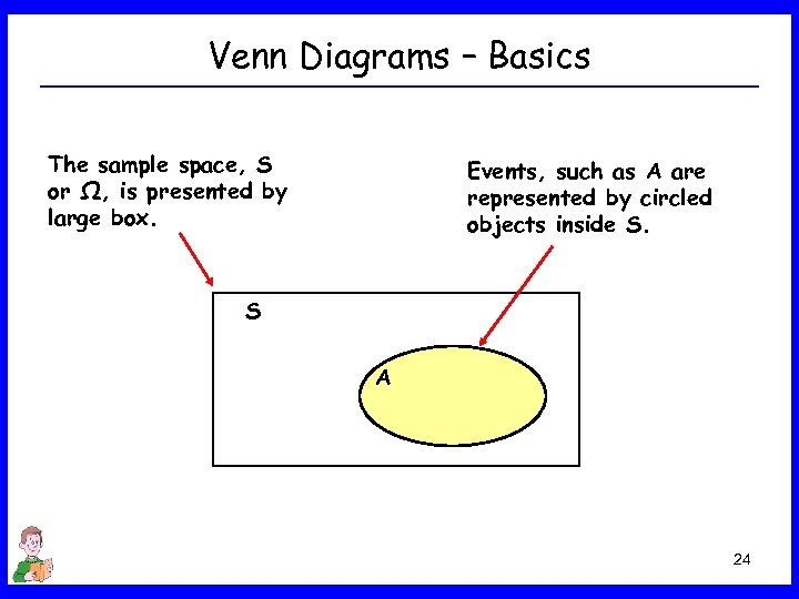Venn Diagrams – Basics The sample space, S or Ω, is presented by large box. Events, such as A are represented by circled objects inside S. S A 24

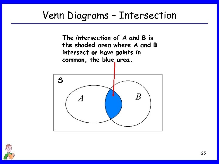Venn Diagrams – Intersection The intersection of A and B is the shaded area where A and B intersect or have points in common, the blue area. S 25

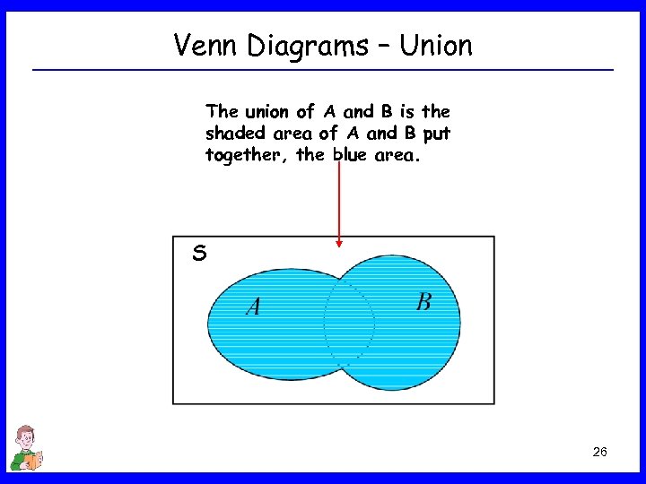Venn Diagrams – Union The union of A and B is the shaded area of A and B put together, the blue area. S 26

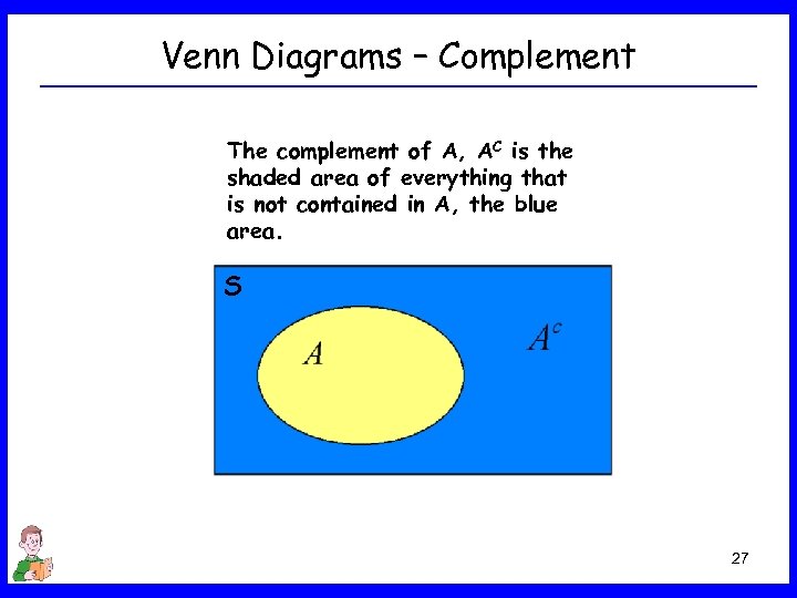Venn Diagrams – Complement The complement of A, AC is the shaded area of everything that is not contained in A, the blue area. S 27

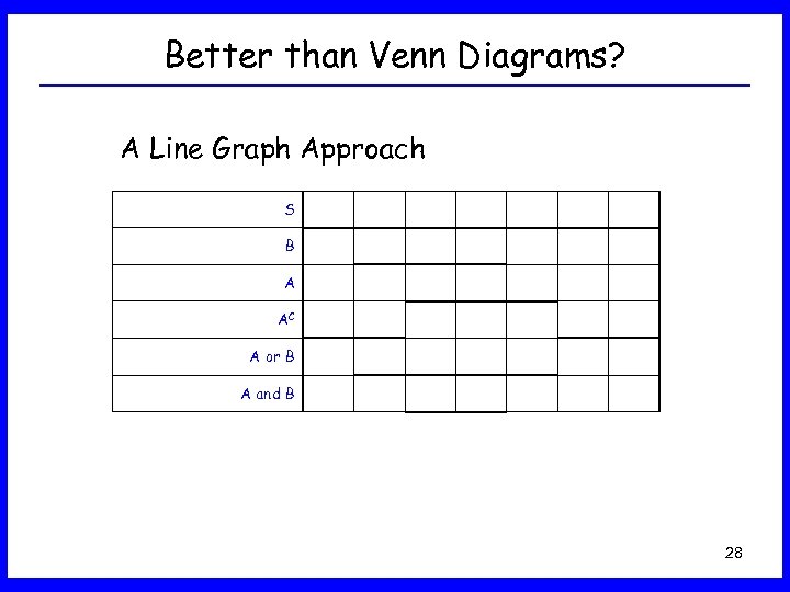Better than Venn Diagrams? A Line Graph Approach S B A AC A or B A and B 28

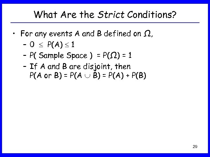What Are the Strict Conditions? • For any events A and B defined on Ω, – 0 P(A) 1 – P( Sample Space ) = P(Ω) = 1 – If A and B are disjoint, then P(A or B) = P(A) + P(B) 29

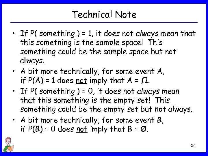Technical Note • If P( something ) = 1, it does not always mean that this something is the sample space! This something could be the sample space but not always. • A bit more technically, for some event A, if P(A) = 1 does not imply that A = Ω. • If P( something ) = 0, it does not always mean that this something is the empty set! This something could be the empty set but not always. • A bit more technically, for some event B, if P(B) = 0 does not imply that B = Ø. 30

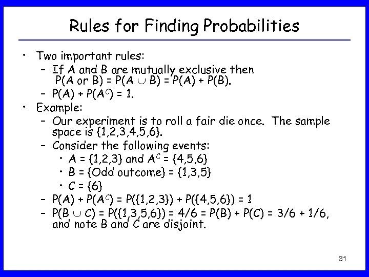Rules for Finding Probabilities • Two important rules: – If A and B are mutually exclusive then P(A or B) = P(A) + P(B). – P(A) + P(AC) = 1. • Example: – Our experiment is to roll a fair die once. The sample space is {1, 2, 3, 4, 5, 6}. – Consider the following events: • A = {1, 2, 3} and AC = {4, 5, 6} • B = {Odd outcome} = {1, 3, 5} • C = {6} – P(A) + P(AC) = P({1, 2, 3}) + P({4, 5, 6}) = 1 – P(B C) = P({1, 3, 5, 6}) = 4/6 = P(B) + P(C) = 3/6 + 1/6, and note B and C are disjoint. 31

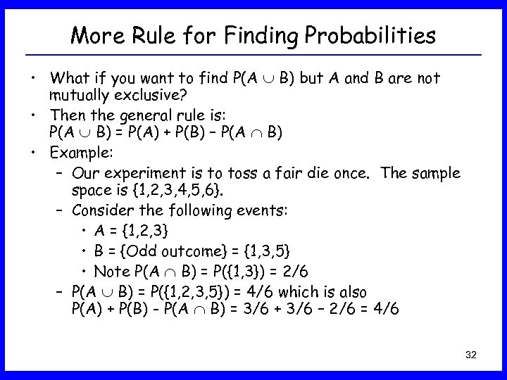More Rule for Finding Probabilities • What if you want to find P(A B) but A and B are not mutually exclusive? • Then the general rule is: P(A B) = P(A) + P(B) – P(A B) • Example: – Our experiment is to toss a fair die once. The sample space is {1, 2, 3, 4, 5, 6}. – Consider the following events: • A = {1, 2, 3} • B = {Odd outcome} = {1, 3, 5} • Note P(A B) = P({1, 3}) = 2/6 – P(A B) = P({1, 2, 3, 5}) = 4/6 which is also P(A) + P(B) - P(A B) = 3/6 + 3/6 – 2/6 = 4/6 32

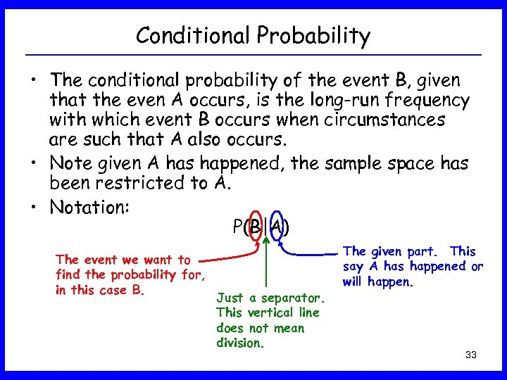Conditional Probability • The conditional probability of the event B, given that the even A occurs, is the long-run frequency with which event B occurs when circumstances are such that A also occurs. • Note given A has happened, the sample space has been restricted to A. • Notation: P(B|A) The event we want to find the probability for, in this case B. Just a separator. This vertical line does not mean division. The given part. This say A has happened or will happen. 33

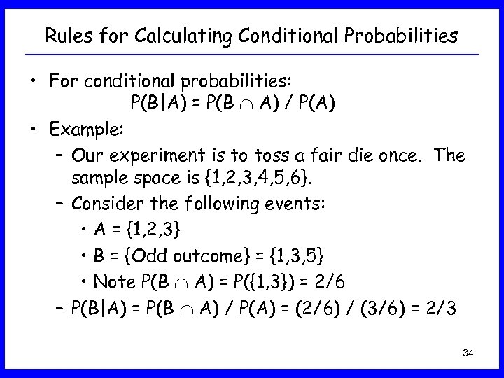Rules for Calculating Conditional Probabilities • For conditional probabilities: P(B|A) = P(B A) / P(A) • Example: – Our experiment is to toss a fair die once. The sample space is {1, 2, 3, 4, 5, 6}. – Consider the following events: • A = {1, 2, 3} • B = {Odd outcome} = {1, 3, 5} • Note P(B A) = P({1, 3}) = 2/6 – P(B|A) = P(B A) / P(A) = (2/6) / (3/6) = 2/3 34

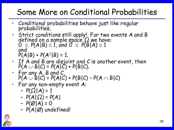Some More on Conditional Probabilities • Conditional probabilities behave just like regular probabilities. • Strict conditions still apply! For two events A and B defined on a sample space Ω we have: 0 P(A|B) 1, and 0 P(B|A) 1 and P(A|B) + P(AC|B) = 1. • If A and B are disjoint and C is another event, then P(A B|C) = P(A|C) + P(B|C). • For any A, B and C, P(A B|C) = P(A|C) + P(B|C) – P(A B|C) • For any non-empty event A: – P(Ω|A) = 1 – P(A|Ω) = P(A) – P(Ø|A) = 0 – P(A|Ø) undefined! 35

Independent/Dependent Events • Two events are independent of each other if knowing that one will occur (or has occurred) will not change the probability of that the other occurs. • Two events are dependent if knowing that one will occur (or has occurred) changes the probability that the other occurs. • Note dependence is about how the probabilities work out when you are given new information. • If the knowledge of occurrence of one event changes the probability of another event then the two events are dependent (not independent. ) 36

Probabilities for Independent Events • If A and B are independent then – P(A B) = P(A) × P(B) – P(A|B) = P(A) (P(B) ≠ 0) – P(B|A) = P(B) (P(A) ≠ 0) • Note using the about relationship you can deduce new ones such as P(A B) = P(A) + P(B) - P(A) × P(B) given that A and B are independent. • Important: What if A and B are not independent and we want to find P(A B)? Then manipulate the definition of conditional probability to get P(A B) = P(A) × P(B|A) = P(A|B) × P(B). 37

Simple Example of Independence • Say you are tossing a fair coin successively. • Then – P(get 2 heads in a row) = P(first toss is head) × P(second toss is head) = ½ × ½ = ¼ – P(get head in the first toss and a tail in the second toss) = P(first toss is head) × P(second toss is tail) = ½ × ½ = ¼ – P(Get a head, then a tail, then a head) = P(first toss is head) × P(second toss is tail) × P(third toss is head) = ½ × ½ = 1/8 38

Example of Dependence • Our experiment is to toss a fair coin 2 times. • The sample space is {HH, HT, TH, TT}. • Are the events A = {HH}, and B = {TT} independent? In other words, P(A B) = P(A) × P(B)? • Let’s see… Note A B = {HH} {TT} = Ø, so P(A B) = P(Ø) = 0 but P(A) × P(B) = P({HH}) × P({TT}) = ¼ × ¼ = 1/16 so Obviously 0 ≠ 1/16! A and B are not independent! • An easier way is to check whether P(A|B) = P(A) holds. You can immediately see that given you have rolled 2 tails, there is no way you could roll 2 heads. Given B happens influences the probability of A happening. 39

Example of Independence • Our experiment is to toss a fair coin 2 times. • The sample space is {HH, HT, TH, TT}. • Are the events A = {first toss is a head} = { HH, HT} B = {second toss is a tail} = {HT, TT} independent? In other words, P(A B) = P(A) × P(B)? • Let’s see… Note A B = {HT} so P(A B) = 1/4 P(A) × P(B) = ½ × ½ = ¼ so A and B are independent! You could have checked P(A|B) = P(A) too. 40

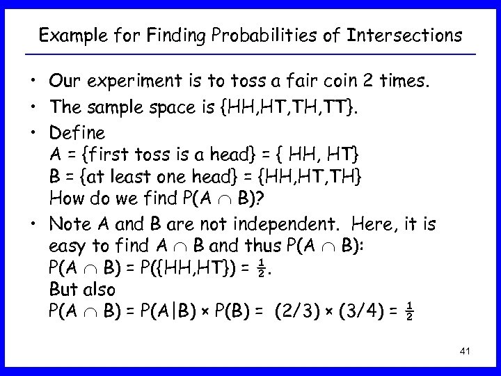Example for Finding Probabilities of Intersections • Our experiment is to toss a fair coin 2 times. • The sample space is {HH, HT, TH, TT}. • Define A = {first toss is a head} = { HH, HT} B = {at least one head} = {HH, HT, TH} How do we find P(A B)? • Note A and B are not independent. Here, it is easy to find A B and thus P(A B): P(A B) = P({HH, HT}) = ½. But also P(A B) = P(A|B) × P(B) = (2/3) × (3/4) = ½ 41

Confusion About Disjoint Events and Independence • Technically, when you want to check to see if A and B are disjoint events, you have to see if A B = Ø. You ask can A and B happen at the same time? • Technically, when you want to check to see if A and B are independent events, you have to see if P(A B) = P(A)×P(B) or P(A|B)=P(A) or P(B|A)=P(B). You ask given one of the events has occurred, does it change the probability of the other event? • Note: – When two events are mutually exclusive and one happens, it turns the probability of the other one to 0. – When two events are independent and one happens, it leaves the probability of the other one alone. 42

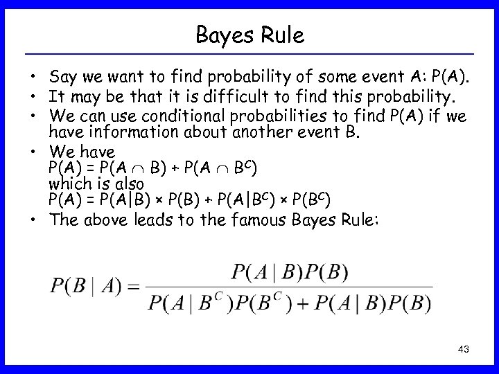Bayes Rule • Say we want to find probability of some event A: P(A). • It may be that it is difficult to find this probability. • We can use conditional probabilities to find P(A) if we have information about another event B. • We have P(A) = P(A B) + P(A BC) which is also P(A) = P(A|B) × P(B) + P(A|BC) × P(BC) • The above leads to the famous Bayes Rule: 43

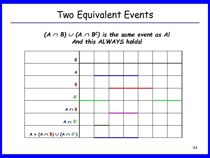Two Equivalent Events (A B) (A BC) is the same event as A! And this ALWAYS holds! S A B BC A = (A B) (A BC) 44

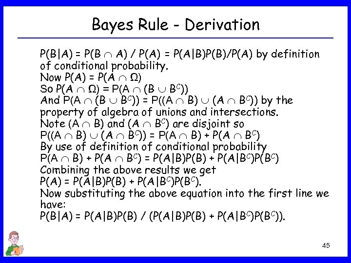Bayes Rule - Derivation P(B|A) = P(B A) / P(A) = P(A|B)P(B)/P(A) by definition of conditional probability. Now P(A) = P(A Ω) So P(A Ω) = P(A (B BC)) And P(A (B BC)) = P((A B) (A BC)) by the property of algebra of unions and intersections. Note (A B) and (A BC) are disjoint so P((A B) (A BC)) = P(A B) + P(A BC) By use of definition of conditional probability P(A B) + P(A BC) = P(A|B)P(B) + P(A|BC)P(BC) Combining the above results we get P(A) = P(A|B)P(B) + P(A|BC)P(BC). Now substituting the above equation into the first line we have: P(B|A) = P(A|B)P(B) / (P(A|B)P(B) + P(A|BC)P(BC)). 45

Application of Probability in Health Sciences • In health sciences field a widely used application of probability is in the evaluation of screening tests and diagnostic criteria. • Of interest is the ability to correctly predict presence or absence of a particular disease from the knowledge of the test (positive or negative) and/or status of presenting symptoms (present or absent). 46

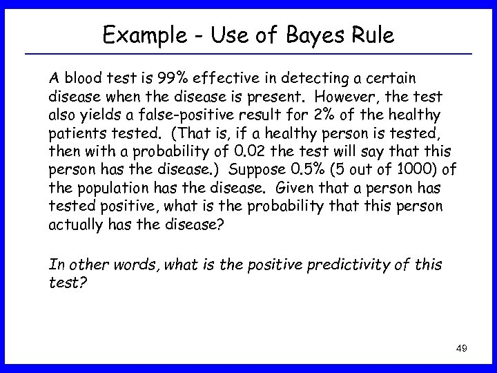
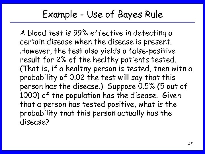Example - Use of Bayes Rule A blood test is 99% effective in detecting a certain disease when the disease is present. However, the test also yields a false-positive result for 2% of the healthy patients tested. (That is, if a healthy person is tested, then with a probability of 0. 02 the test will say that this person has the disease. ) Suppose 0. 5% (5 out of 1000) of the population has the disease. Given that a person has tested positive, what is the probability that this person actually has the disease? 47

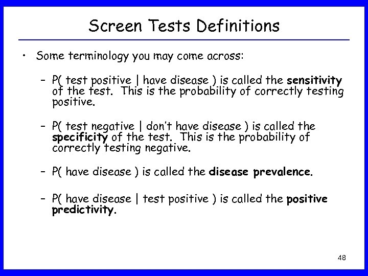Screen Tests Definitions • Some terminology you may come across: – P( test positive | have disease ) is called the sensitivity of the test. This is the probability of correctly testing positive. – P( test negative | don’t have disease ) is called the specificity of the test. This is the probability of correctly testing negative. – P( have disease ) is called the disease prevalence. – P( have disease | test positive ) is called the positive predictivity. 48

Example - Use of Bayes Rule A blood test is 99% effective in detecting a certain disease when the disease is present. However, the test also yields a false-positive result for 2% of the healthy patients tested. (That is, if a healthy person is tested, then with a probability of 0. 02 the test will say that this person has the disease. ) Suppose 0. 5% (5 out of 1000) of the population has the disease. Given that a person has tested positive, what is the probability that this person actually has the disease? In other words, what is the positive predictivity of this test? 49

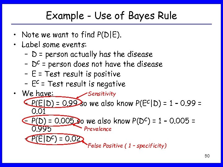Example - Use of Bayes Rule • Note we want to find P(D|E). • Label some events: – D = person actually has the disease – DC = person does not have the disease – E = Test result is positive – EC = Test result is negative Sensitivity • We have: – P(E|D) = 0. 99 so we also know P(EC|D) = 1 – 0. 99 = 0. 01 – P(D) = 0. 005 so we also know P(DC) = 1 – 0. 005 = Prevalence 0. 995 – P(E|DC) = 0. 02 False Positive ( 1 – specificity) 50

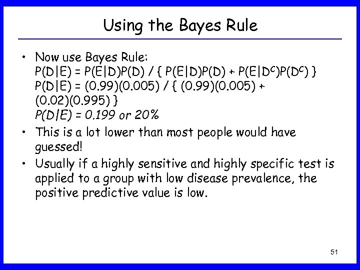Using the Bayes Rule • Now use Bayes Rule: P(D|E) = P(E|D)P(D) / { P(E|D)P(D) + P(E|DC)P(DC) } P(D|E) = (0. 99)(0. 005) / { (0. 99)(0. 005) + (0. 02)(0. 995) } P(D|E) = 0. 199 or 20% • This is a lot lower than most people would have guessed! • Usually if a highly sensitive and highly specific test is applied to a group with low disease prevalence, the positive predictive value is low. 51

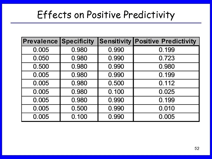Effects on Positive Predictivity 52

What is a Random Variable? • Random Variable: assigns a number to each outcome of a random circumstance, or, equivalently, to each unit in a population. • Two different broad classes of random variables: 1. A continuous random variable can take any value in an interval or collection of intervals. 2. A discrete random variable can take one of a countable list of distinct values. 53

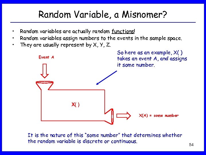Random Variable, a Misnomer? • • • Random variables are actually random functions! Random variables assign numbers to the events in the sample space. They are usually represent by X, Y, Z. So here as an example, X( ) Event A takes an event A, and assigns it some number. X( ) X(A) = some number It is the nature of this “some number” that determines whether the random variable is discrete or continuous. 54

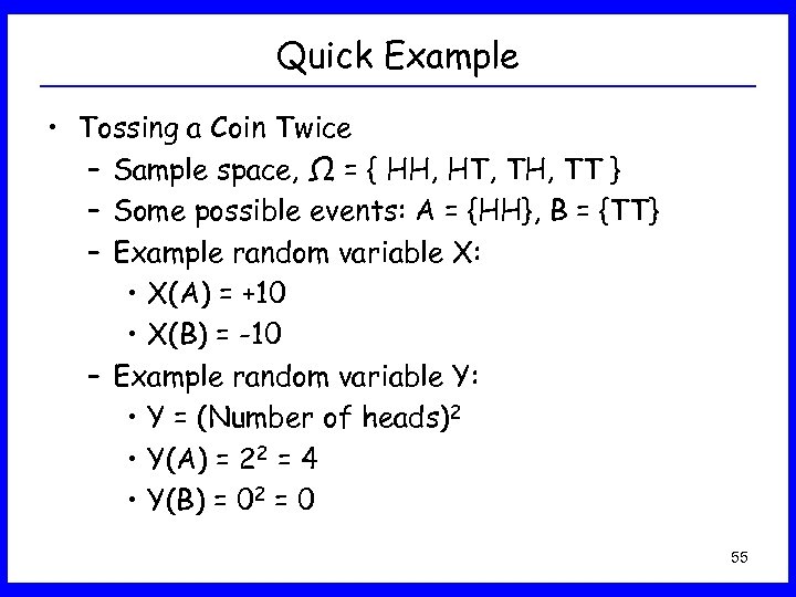Quick Example • Tossing a Coin Twice – Sample space, Ω = { HH, HT, TH, TT } – Some possible events: A = {HH}, B = {TT} – Example random variable X: • X(A) = +10 • X(B) = -10 – Example random variable Y: • Y = (Number of heads)2 • Y(A) = 22 = 4 • Y(B) = 02 = 0 55

Why would you need random variable? • You are quite often interested in some function of an event and not in the event itself. • Example: – Consider a game where you toss a fair coin twice. You win $5 when a head comes up and lose $5 when a tail comes up. The sample space, Ω, is { HH, HT, TH, TT }. • Some possible events: A = {HH}, B = {TT} • Here X(A) = 5 + 5 = 10 & X(B) = -5 – 5 = -10. • Now instead of asking P(A), what is the probability you get two heads in a row, you ask P(X = 10), what is the probability you win $10. – You could ask questions like • P( 0 ≤ X ≤ 5), what is the probability you win between zero and $5, inclusive. • P( X > 3), what is the probability you win more than $3. • Etc. 56

Discrete Random Variables • Notation: – X, the random variable. Note X means X(some event) but the “(some event)” part is quite often repressed. – P(X = k), probability that X takes on the value k, where k is one of the possible values of X. • Discrete random variable: can only result in a countable set of possibilities – often a finite number of outcomes, but can be infinite (e. g. tossing a coin an infinite number of times. ) 57

Probability Distribution Function • Probability distribution function (pdf) of X is a table or rule that assigns probabilities to possible values of X. • How do you find pdf of X? 1. List all simple events in sample space. 2. Find probability for each simple event. 3. List possible values for random variable X and identify the value for each simple event. 4. Find all simple events for which X = k, for each possible value k. 5. P(X = k) is the sum of the probabilities for all simple events for which X = k. 58

Conditions for pdf of X discrete • Condition 1 - The sum of the probabilities over all possible values of a discrete random variable must equal 1. • Condition 2 - The probability of any specific outcome for a discrete random variable must be between 0 and 1. 59

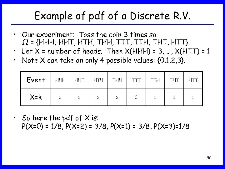Example of pdf of a Discrete R. V. • Our experiment: Toss the coin 3 times so Ω = {HHH, HHT, HTH, THH, TTT, TTH, THT, HTT} • Let X = number of heads. Then X(HHH) = 3, …, X(HTT) = 1 • Note X can take on only 4 possible values: {0, 1, 2, 3}. Event HHH HHT HTH THH TTT TTH THT HTT X=k 3 2 2 2 0 1 1 1 • So here the pdf of X is: P(X=0) = 1/8, P(X=2) = 3/8, P(X=1) = 3/8, P(X=3)=1/8 60

Cumulative Distribution Function (CDF) • Cumulative distribution function (cdf) for a random variable X is a rule or table that provides the probabilities P(X ≤ k) for any real number k. • Cumulative probability = probability that X is less than or equal to a particular value. • These definitions hold for both discrete and continuous variables. 61

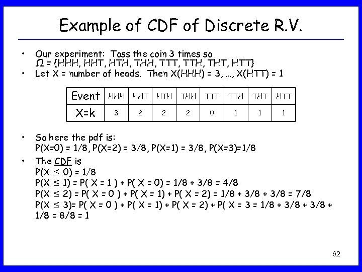Example of CDF of Discrete R. V. • • Our experiment: Toss the coin 3 times so Ω = {HHH, HHT, HTH, THH, TTT, TTH, THT, HTT} Let X = number of heads. Then X(HHH) = 3, …, X(HTT) = 1 Event • HHT HTH THH TTT TTH THT HTT X=k • HHH 3 2 2 2 0 1 1 1 So here the pdf is: P(X=0) = 1/8, P(X=2) = 3/8, P(X=1) = 3/8, P(X=3)=1/8 The CDF is P(X ≤ 0) = 1/8 P(X ≤ 1) = P( X = 1 ) + P( X = 0) = 1/8 + 3/8 = 4/8 P(X ≤ 2) = P( X = 0 ) + P( X = 1) + P( X = 2) = 1/8 + 3/8 = 7/8 P(X ≤ 3)= P( X = 0 ) + P( X = 1) + P( X = 2) + P( X = 3 = 1/8 + 3/8 + 1/8 = 8/8 = 1 62

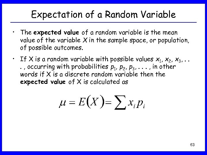Expectation of a Random Variable • The expected value of a random variable is the mean value of the variable X in the sample space, or population, of possible outcomes. • If X is a random variable with possible values x 1, x 2, x 3, . . . , occurring with probabilities p 1, p 2, p 3, . . . , in other words if X is a discrete random variable then the expected value of X is calculated as 63

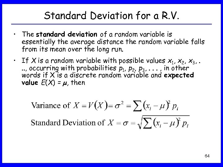Standard Deviation for a R. V. • The standard deviation of a random variable is essentially the average distance the random variable falls from its mean over the long run. • If X is a random variable with possible values x 1, x 2, x 3, . . . , occurring with probabilities p 1, p 2, p 3, . . . , in other words if X is a discrete random variable and expected value E(X) = , then 64

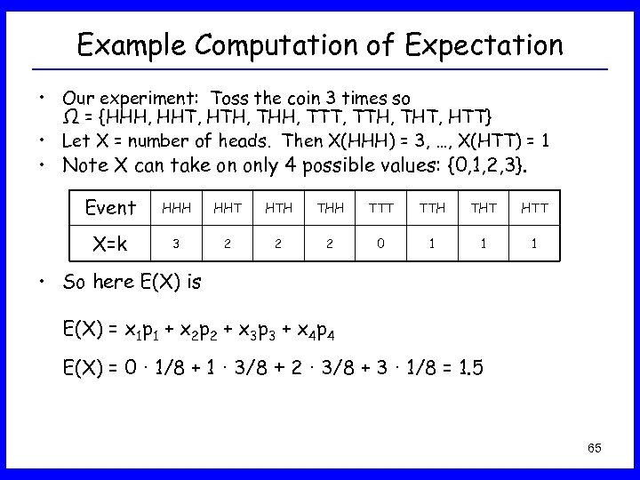Example Computation of Expectation • Our experiment: Toss the coin 3 times so Ω = {HHH, HHT, HTH, THH, TTT, TTH, THT, HTT} • Let X = number of heads. Then X(HHH) = 3, …, X(HTT) = 1 • Note X can take on only 4 possible values: {0, 1, 2, 3}. Event HHH HHT HTH THH TTT TTH THT HTT X=k 3 2 2 2 0 1 1 1 • So here E(X) is E(X) = x 1 p 1 + x 2 p 2 + x 3 p 3 + x 4 p 4 E(X) = 0 · 1/8 + 1 · 3/8 + 2 · 3/8 + 3 · 1/8 = 1. 5 65

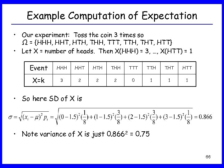Example Computation of Expectation • Our experiment: Toss the coin 3 times so Ω = {HHH, HHT, HTH, THH, TTT, TTH, THT, HTT} • Let X = number of heads. Then X(HHH) = 3, …, X(HTT) = 1 Event HHH HHT HTH THH TTT TTH THT HTT X=k 3 2 2 2 0 1 1 1 • So here SD of X is • Note variance of X is just 0. 8662 = 0. 75 66

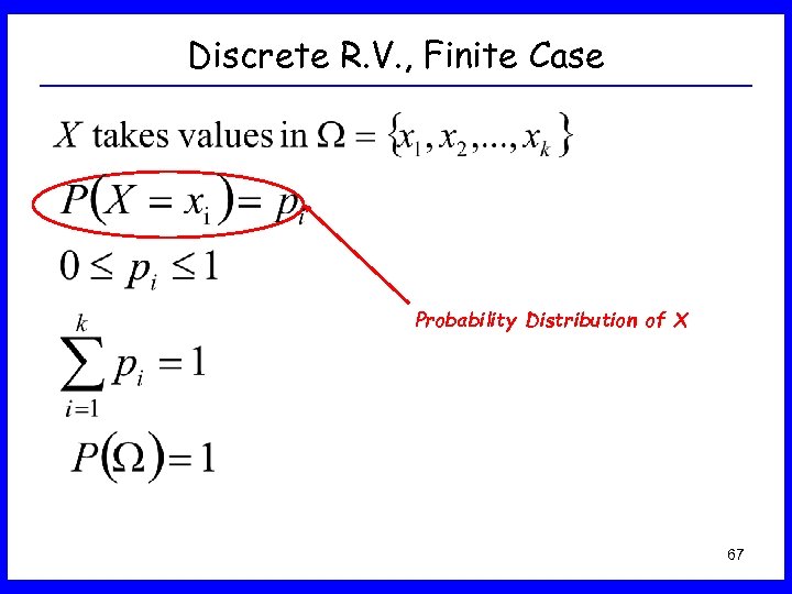Discrete R. V. , Finite Case Probability Distribution of X 67

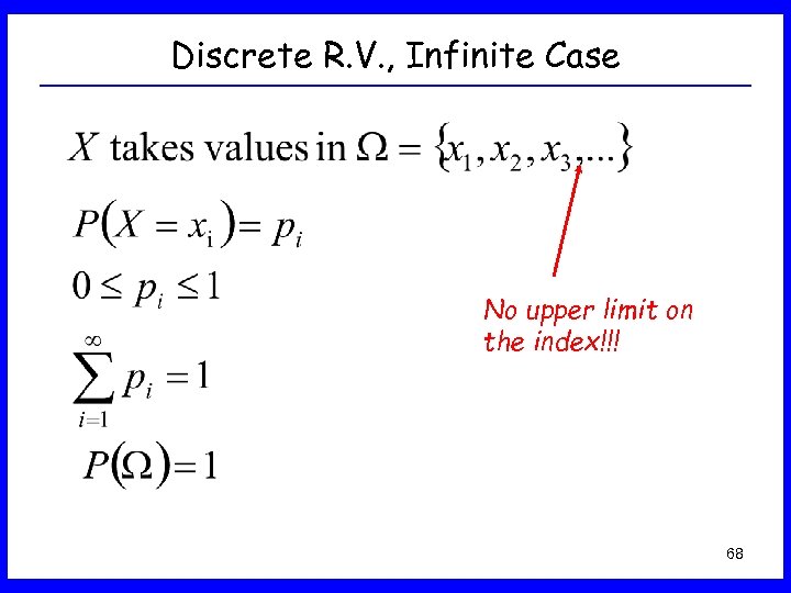Discrete R. V. , Infinite Case No upper limit on the index!!! 68

Special Discrete R. V. s • You can categorize discrete random variables: – Binomial – Poisson – Bernoulli – Geometric – Hypergeometric – Negative binomial – Uniform Discrete • All of the above random variables have countable set of values 69

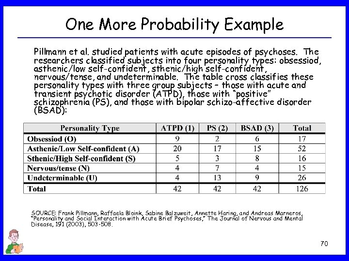One More Probability Example Pillmann et al. studied patients with acute episodes of psychoses. The researchers classified subjects into four personality types: obsessiod, asthenic/low self-confident, sthenic/high self-confident, nervous/tense, and undeterminable. The table cross classifies these personality types with three group subjects – those with acute and transient psychotic disorder (ATPD), those with “positive” schizophrenia (PS), and those with bipolar schizo-affective disorder (BSAD): SOURCE: Frank Pillmann, Raffaela Bloink, Sabine Balzuweit, Annette Haring, and Andreas Marneros, “Personality and Social Interaction with Acute Brief Psychoses, ” The Journal of Nervous and Mental Disease, 191 (2003), 503 -508. 70

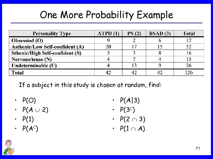One More Probability Example If a subject in this study is chosen at random, find: • • P(O) P(A 2) P(1) P(AC) • • P(A|3) P(3 C) P(2 3) P(1 A) 71

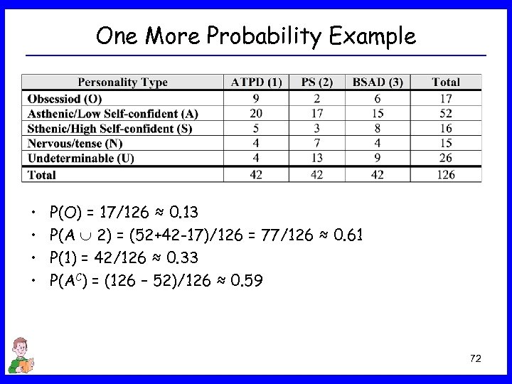One More Probability Example • • P(O) = 17/126 ≈ 0. 13 P(A 2) = (52+42 -17)/126 = 77/126 ≈ 0. 61 P(1) = 42/126 ≈ 0. 33 P(AC) = (126 – 52)/126 ≈ 0. 59 72

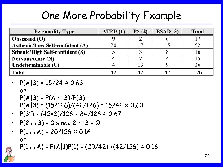One More Probability Example • P(A|3) = 15/24 ≈ 0. 63 or P(A|3) = P(A 3)/P(3) P(A|3) = (15/126)/(42/126) = 15/42 ≈ 0. 63 • P(3 C) = (42× 2)/126 = 84/126 ≈ 0. 67 • P(2 3) = 0 since 2 3 = Ø • P(1 A) = 20/126 ≈ 0. 16 or P(1 A) = P(A|1)P(1) = (20/42) ×(42/126) ≈ 0. 16 73

Continuous Random Variables • Continuous random variable: the outcome can be any value in an interval or collection of intervals. • Probability density function for a continuous random variable X is a curve such that the area under the curve over an interval equals the probability that X is in that interval. P(a X b) = area under density curve over the interval between the values a and b. • The cumulative density function is defined as P(X t) = area to the left of t. 74

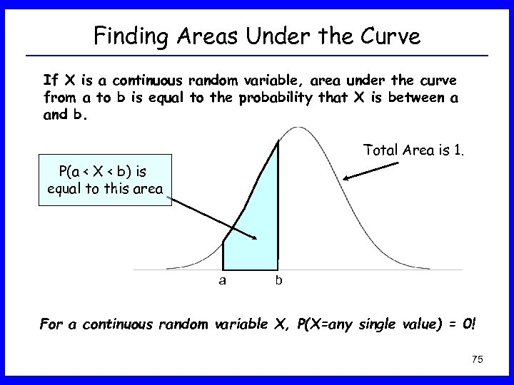Finding Areas Under the Curve If X is a continuous random variable, area under the curve from a to b is equal to the probability that X is between a and b. Total Area is 1. P(a < X < b) is equal to this area a b For a continuous random variable X, P(X=any single value) = 0! 75

Normal Random Variable • Perhaps the most famous continuous random variable is the Normal (Gaussian) Random variable. • It is characterized by two numbers: – Its mean, – And its standard deviation, • If X is a normal random variable then the shorthand is X ~ N( , 2) • X is called the standard normal random variable if X ~ N( =0, 2=1). It is often represented by Z. 76

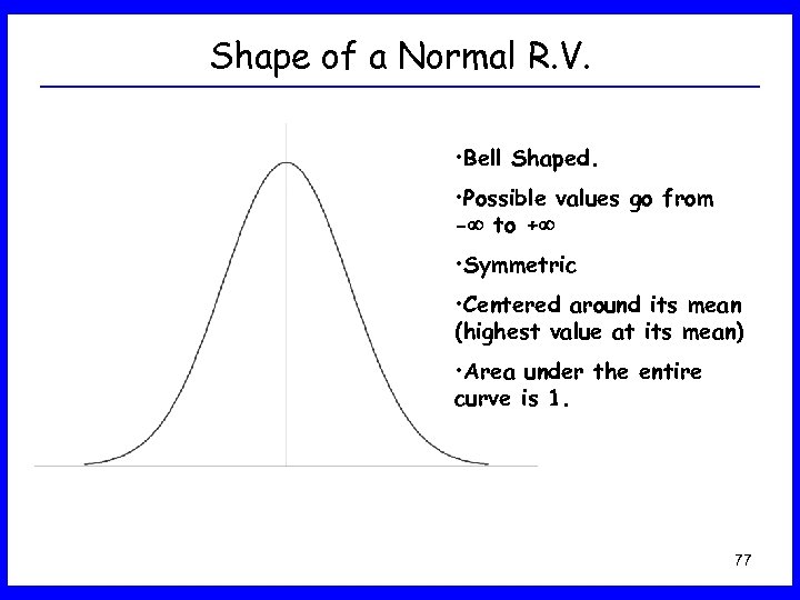Shape of a Normal R. V. • Bell Shaped. • Possible values go from - to + • Symmetric • Centered around its mean (highest value at its mean) • Area under the entire curve is 1. 77

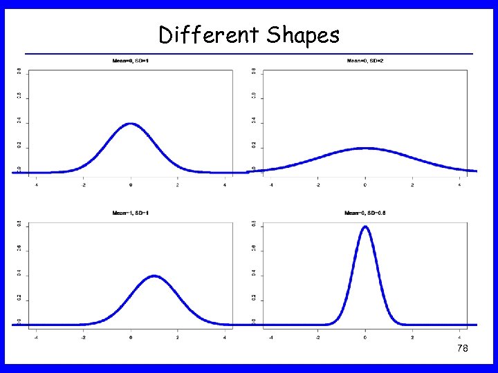Different Shapes 78

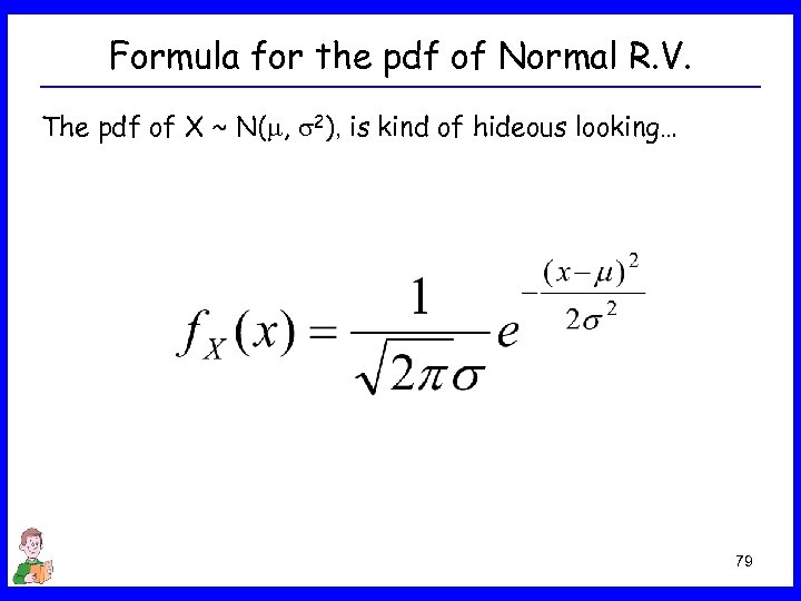Formula for the pdf of Normal R. V. The pdf of X ~ N( , 2), is kind of hideous looking… 79

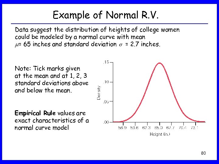Example of Normal R. V. Data suggest the distribution of heights of college women could be modeled by a normal curve with mean = 65 inches and standard deviation = 2. 7 inches. Note: Tick marks given at the mean and at 1, 2, 3 standard deviations above and below the mean. Empirical Rule values are exact characteristics of a normal curve model 80

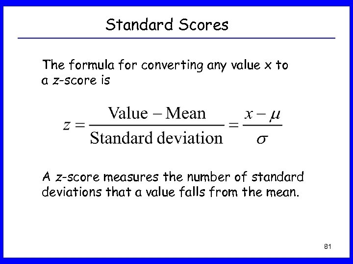Standard Scores The formula for converting any value x to a z-score is A z-score measures the number of standard deviations that a value falls from the mean. 81

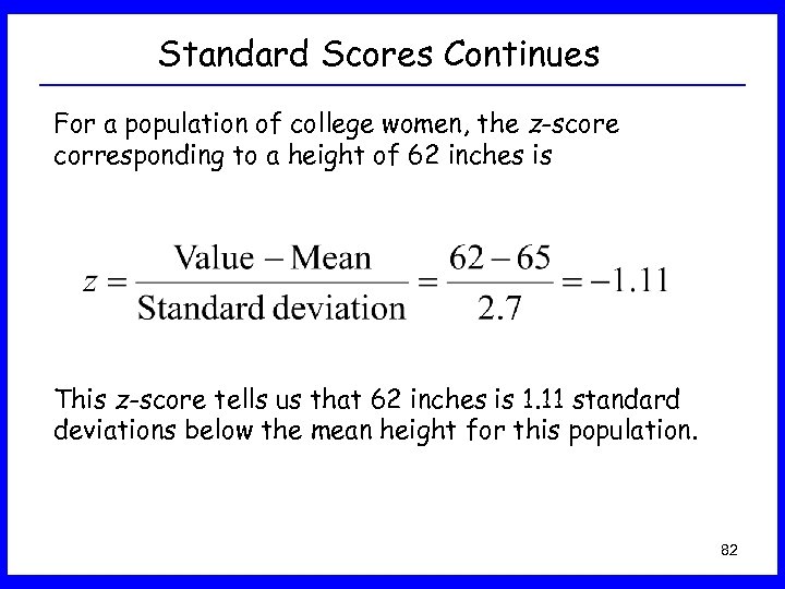Standard Scores Continues For a population of college women, the z-score corresponding to a height of 62 inches is This z-score tells us that 62 inches is 1. 11 standard deviations below the mean height for this population. 82

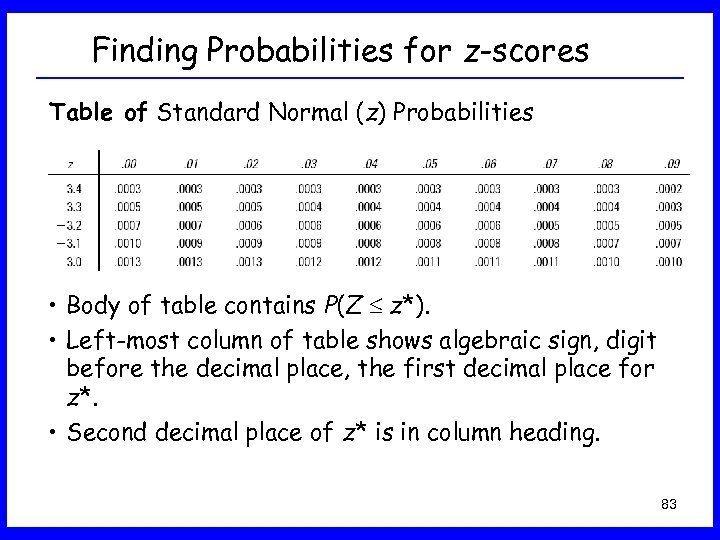Finding Probabilities for z-scores Table of Standard Normal (z) Probabilities • Body of table contains P(Z z*). • Left-most column of table shows algebraic sign, digit before the decimal place, the first decimal place for z*. • Second decimal place of z* is in column heading. 83

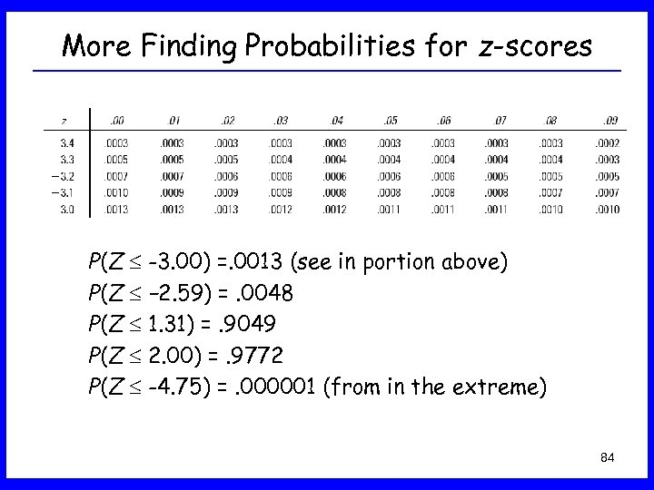More Finding Probabilities for z-scores P(Z -3. 00) =. 0013 (see in portion above) P(Z − 2. 59) =. 0048 P(Z 1. 31) =. 9049 P(Z 2. 00) =. 9772 P(Z -4. 75) =. 000001 (from in the extreme) 84

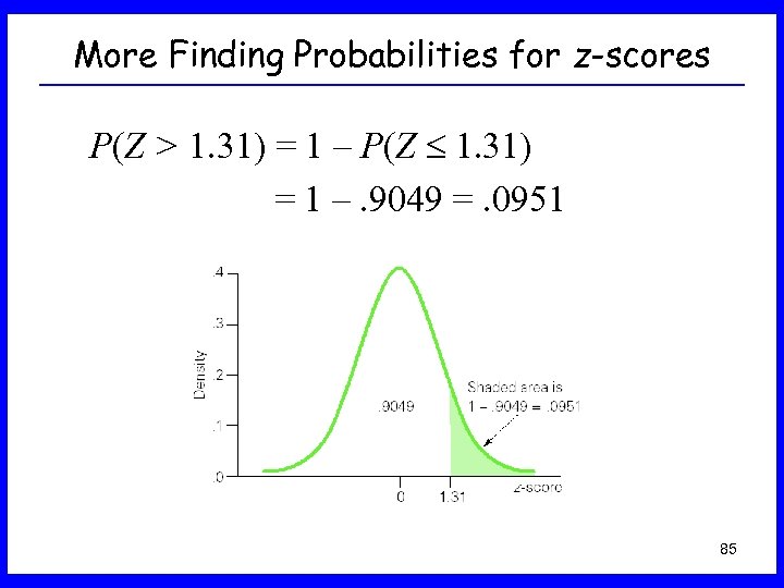More Finding Probabilities for z-scores P(Z > 1. 31) = 1 – P(Z 1. 31) = 1 –. 9049 =. 0951 85

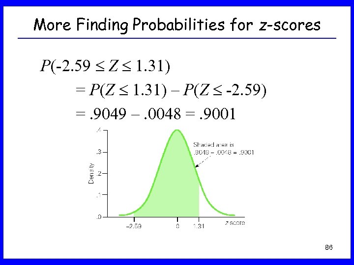More Finding Probabilities for z-scores P(-2. 59 Z 1. 31) = P(Z 1. 31) – P(Z -2. 59) =. 9049 –. 0048 =. 9001 86

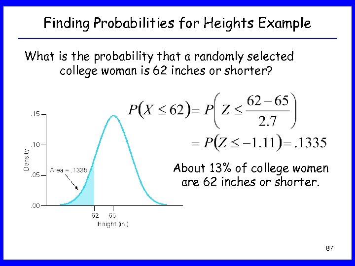Finding Probabilities for Heights Example What is the probability that a randomly selected college woman is 62 inches or shorter? About 13% of college women are 62 inches or shorter. 87

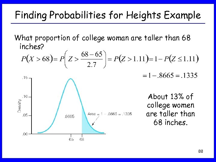Finding Probabilities for Heights Example What proportion of college woman are taller than 68 inches? About 13% of college women are taller than 68 inches. 88

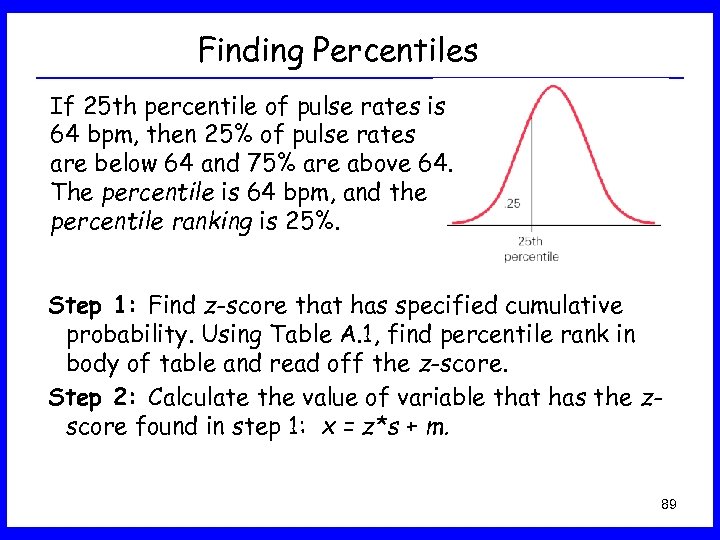Finding Percentiles If 25 th percentile of pulse rates is 64 bpm, then 25% of pulse rates are below 64 and 75% are above 64. The percentile is 64 bpm, and the percentile ranking is 25%. Step 1: Find z-score that has specified cumulative probability. Using Table A. 1, find percentile rank in body of table and read off the z-score. Step 2: Calculate the value of variable that has the zscore found in step 1: x = z*s + m. 89

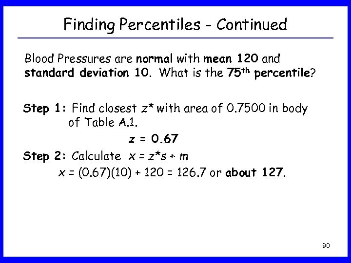Finding Percentiles - Continued Blood Pressures are normal with mean 120 and standard deviation 10. What is the 75 th percentile? Step 1: Find closest z* with area of 0. 7500 in body of Table A. 1. z = 0. 67 Step 2: Calculate x = z*s + m x = (0. 67)(10) + 120 = 126. 7 or about 127. 90

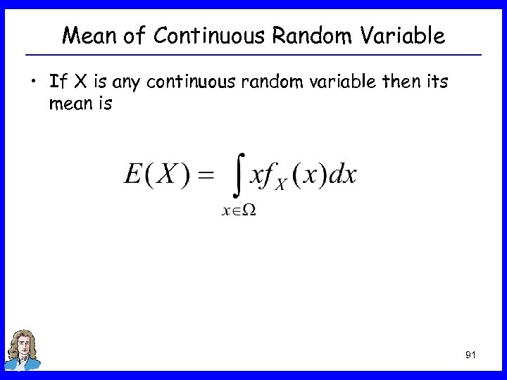Mean of Continuous Random Variable • If X is any continuous random variable then its mean is 91

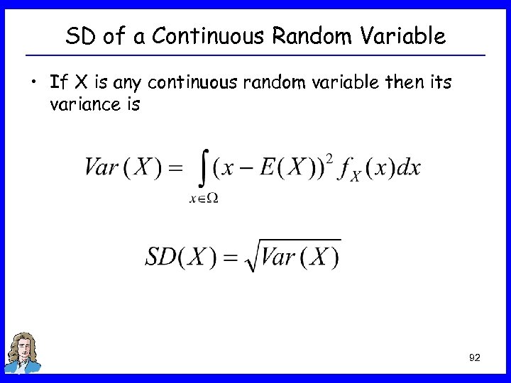SD of a Continuous Random Variable • If X is any continuous random variable then its variance is 92

Special Continuous R. V. s • You can categorize continuous random variables: – Normal – Uniform – Exponential – Gamma – Beta • All of the above random variables have uncountable set of values 93

Sums, Differences, Combinations of R. V. s A linear combination of random variables, X, Y, . . . is a combination of the form: L = a. X + b. Y + … where a, b, etc. are numbers – positive or negative. Most common: Sum = X + Y Difference = X – Y 94

Means of Linear Combinations The mean of L is: Mean(L) = a Mean(X) + b Mean(Y) + … Most common: Mean( X + Y) = Mean(X) + Mean(Y) Mean(X – Y) = Mean(X) – Mean(Y) 95

Independence of R. V. s • Independence of two or more random variables is very similar to the independence of two or more event. • Independence means that knowing something about the value of X tells knowing about the probabilities for Y. • “X and Y independent” means that the events {a < X < b} and {c < Y < d} are independent for all numbers a, b, c, and d so P({a < X < b} and {c < Y < d} ) = P({a < X < b})·P({c < Y < d}) 96

Variances of Linear Combinations If X, Y, . . . are independent random variables, then Variance(L) = a 2 Variance(X) + b 2 Variance(Y) + … Most common: Variance( X + Y) = Variance(X) + Variance(Y) Variance(X – Y) = Variance(X) + Variance(Y) 97

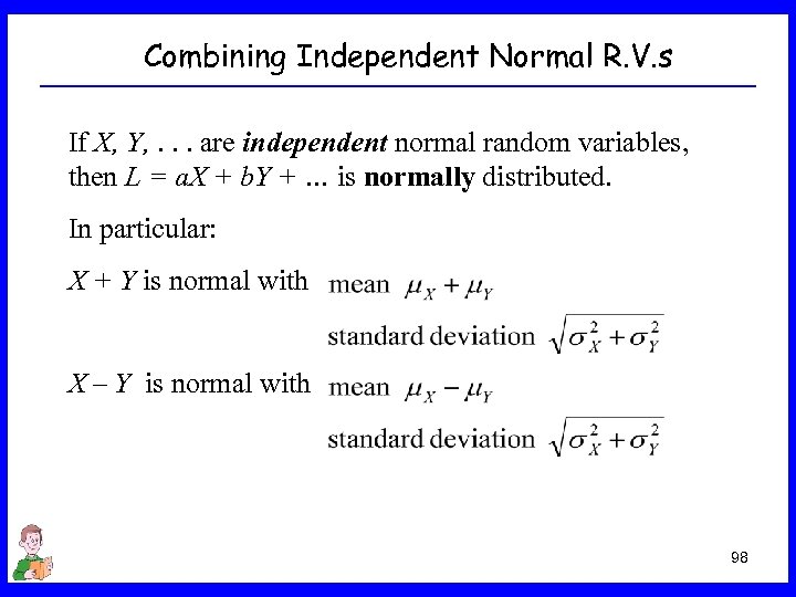Combining Independent Normal R. V. s If X, Y, . . . are independent normal random variables, then L = a. X + b. Y + … is normally distributed. In particular: X + Y is normal with X – Y is normal with 98