Welcome to EC 209 Managerial Economics- Group A

Welcome to EC 209: Managerial Economics- Group A By: Dr. Jacqueline Khorassani Week Seven 1

Managerial Economics Week Seven- Class 1 Monday, October 15 11: 10 -12: 00 Fottrell (AM) 2

This week’s Aplia Assignment IS DUE BEFORE 5: 00 PM Wednesday You did not send me any questions Should I assume you are ok? 3

Long Run Production Function n What is long run? – All factor of production are variable – In our example we had K and L – We can hire more of both – This is the planning stage of production – How big the plant should be? 4

Isoquant n A curve that shows the combinations of inputs (K, L) that yield the same level of output. n Suppose our goal is to produce 100 widgets per day – What combinations of K and L yield 100 widgets per day? 5

How does an isoquant look? n The shape depends upon: K 1. the state of technical knowledge, and 2. the degree of substitution between factors. L 6

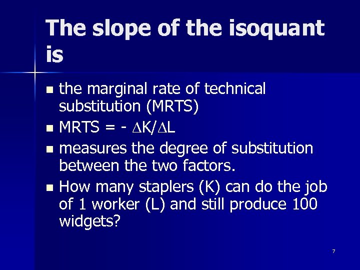The slope of the isoquant is the marginal rate of technical substitution (MRTS) n MRTS = - DK/DL n measures the degree of substitution between the two factors. n How many staplers (K) can do the job of 1 worker (L) and still produce 100 widgets? n 7

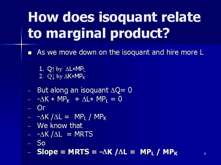How does isoquant relate to marginal product? n As we move down on the isoquant and hire more L 1. 2. – – – – Q↑ by DL*MPL Q↓ by DK*MPK But along an isoquant DQ= 0 -DK * MPK + DL* MPL = 0 Or -DK /DL = MPL / MPK We know that -DK /DL = MRTS So Slope = MRTS = -DK /DL = MPL / MPK 8

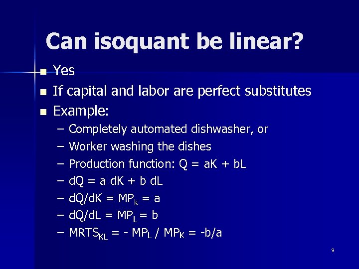Can isoquant be linear? n n n Yes If capital and labor are perfect substitutes Example: – – – – Completely automated dishwasher, or Worker washing the dishes Production function: Q = a. K + b. L d. Q = a d. K + b d. L d. Q/d. K = MPk = a d. Q/d. L = MPL = b MRTSKL = - MPL / MPK = -b/a 9

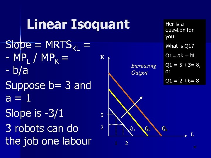Linear Isoquant Slope = MRTSKL = - MPL / MPK = - b/a Suppose b= 3 and a = 1 Slope is -3/1 3 robots can do the job one labour Her is a question for you What is Q 1? Q 1= ak + b. L K Increasing Output Q 1 = 5 +3= 8, or Q 1 = 2 +6= 8 5 2 Q 1 1 2 Q 3 L 10

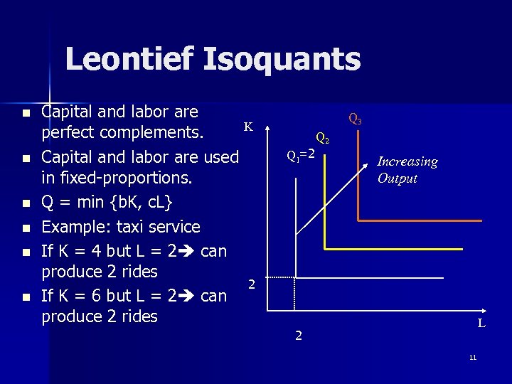Leontief Isoquants n n n Capital and labor are K perfect complements. Capital and labor are used in fixed-proportions. Q = min {b. K, c. L} Example: taxi service If K = 4 but L = 2 can produce 2 rides 2 If K = 6 but L = 2 can produce 2 rides Q 3 Q 1=2 Q 2 Increasing Output L 2 11

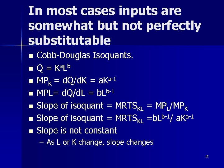In most cases inputs are somewhat but not perfectly substitutable n n n n Cobb-Douglas Isoquants. Q = Ka. Lb MPK = d. Q/d. K = a. Ka-1 MPL= d. Q/d. L = b. Lb-1 Slope of isoquant = MRTSKL = MPL/MPK Slope of isoquant = MRTSKL =b. Lb-1/ a. Ka-1 Slope is not constant – As L or K change, slope changes 12

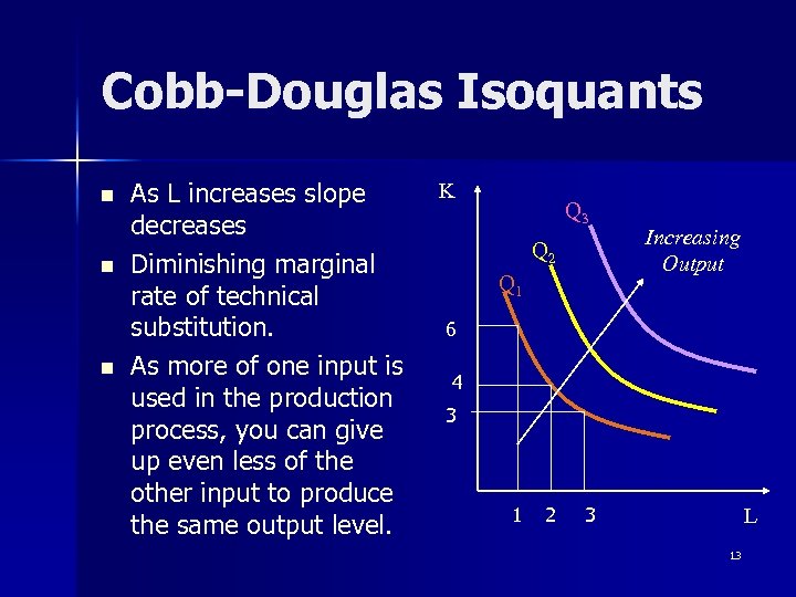Cobb-Douglas Isoquants n n n As L increases slope decreases Diminishing marginal rate of technical substitution. As more of one input is used in the production process, you can give up even less of the other input to produce the same output level. K Q 3 Q 2 Q 1 Increasing Output 6 4 3 1 2 3 L 13

So you know your isoquant n n You decide that you want to produce Q 1 amount of output What combination of K and L are you going to hire? It depends on What combination of K and L minimizes your cost n What is the price of labour and capital? 14

Total cost of production Is the cost of capital plus the cost of labour n Total cost = TC = r. K + w. L where n r = payment to a unit of capital w = payment to a unit of labour 15

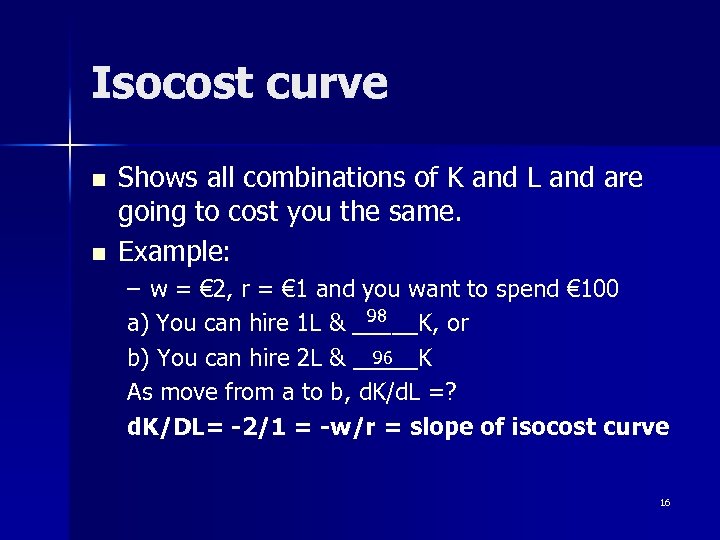Isocost curve n n Shows all combinations of K and L and are going to cost you the same. Example: – w = € 2, r = € 1 and you want to spend € 100 98 a) You can hire 1 L & _____K, or 96 b) You can hire 2 L & _____K As move from a to b, d. K/d. L =? d. K/DL= -2/1 = -w/r = slope of isocost curve 16

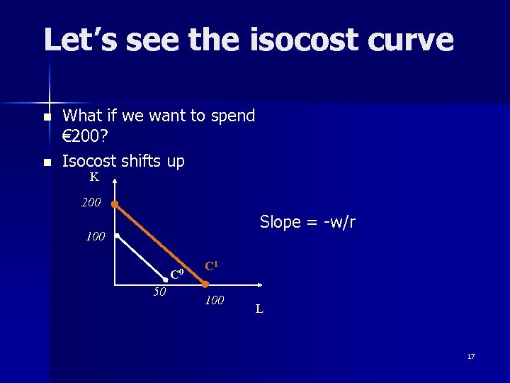Let’s see the isocost curve n n What if we want to spend € 200? Isocost shifts up K 200 Slope = -w/r 100 C 0 50 C 1 100 L 17

Managerial Economics. Group A n Week Seven- Class 2 – Tuesday, October 16 – Cairnes – 15: 10 -16: 00 n Aplia assignment is due before 5 PM tomorrow 18

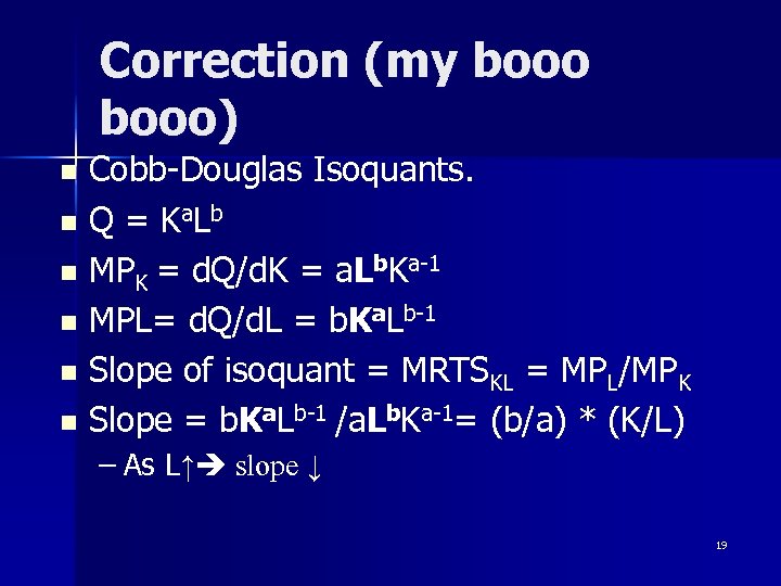Correction (my booo) Cobb-Douglas Isoquants. n Q = Ka. Lb n MPK = d. Q/d. K = a. Lb. Ka-1 n MPL= d. Q/d. L = b. Ka. Lb-1 n Slope of isoquant = MRTSKL = MPL/MPK n Slope = b. Ka. Lb-1 /a. Lb. Ka-1= (b/a) * (K/L) n – As L↑ slope ↓ 19

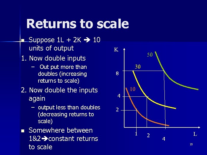Returns to scale Suppose 1 L + 2 K 10 units of output 1. Now double inputs n – Out put more than doubles (increasing returns to scale) 2. Now double the inputs again – output less than doubles (decreasing returns to scale) n Somewhere between 1&2 constant returns to scale K 50 30 8 10 4 2 1 2 L 4 20

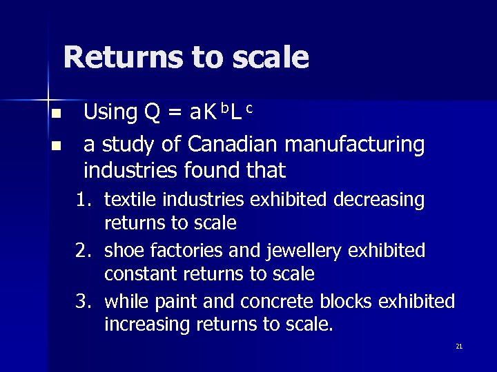Returns to scale n n Using Q = a K b L c a study of Canadian manufacturing industries found that 1. textile industries exhibited decreasing returns to scale 2. shoe factories and jewellery exhibited constant returns to scale 3. while paint and concrete blocks exhibited increasing returns to scale. 21

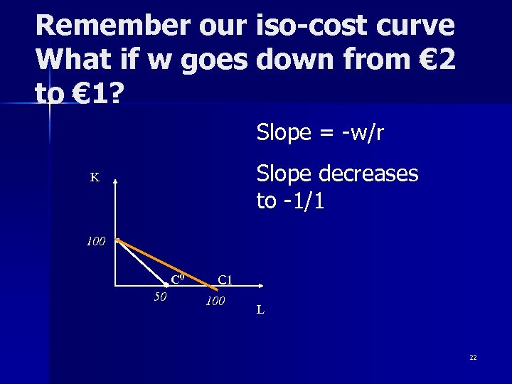Remember our iso-cost curve What if w goes down from € 2 to € 1? Slope = -w/r Slope decreases to -1/1 K 100 C 0 50 C 1 100 L 22

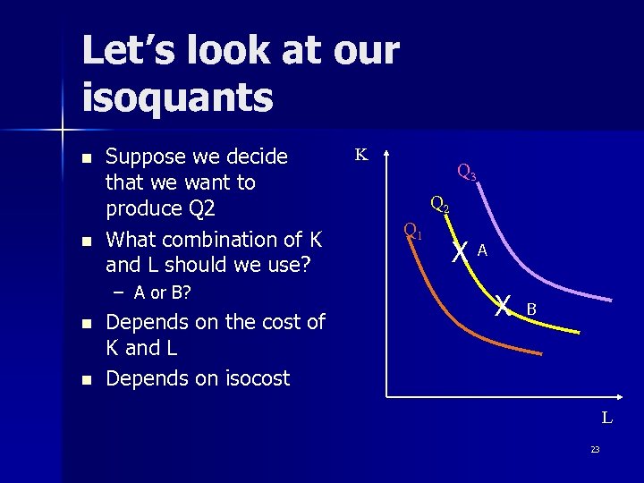Let’s look at our isoquants n n Suppose we decide that we want to produce Q 2 What combination of K and L should we use? – A or B? n n Depends on the cost of K and L Depends on isocost K Q 3 Q 2 Q 1 X A X B L 23

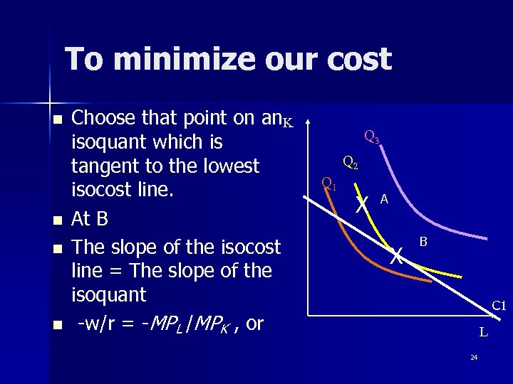To minimize our cost n n Choose that point on an K isoquant which is tangent to the lowest isocost line. At B The slope of the isocost line = The slope of the isoquant -w/r = -MPL /MPK , or Q 3 Q 2 Q 1 X A X B C 1 L 24

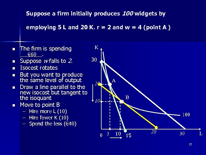Suppose a firm initially produces 100 widgets by employing 5 L and 20 K. r = 2 and w = 4 (point A ) n n n The firm is spending _______. € 60 Suppose w falls to 2. Isocost rotates But you want to produce the same level of output Draw a line parallel to the new isocost but tangent to the isoquant Move to point B – – – K 30 A 20 B 10 Hire more L (10) Hire fewer K (10) Spend the less (€ 40) Spend the less ( 100 0 5 10 15 20 30 L 25

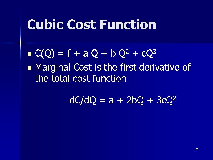Cubic Cost Function C(Q) = f + a Q + b Q 2 + c. Q 3 n Marginal Cost is the first derivative of the total cost function n d. C/d. Q = a + 2 b. Q + 3 c. Q 2 26

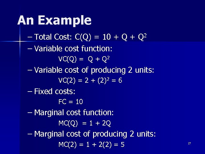An Example – Total Cost: C(Q) = 10 + Q 2 – Variable cost function: VC(Q) = Q + Q 2 – Variable cost of producing 2 units: VC(2) = 2 + (2)2 = 6 – Fixed costs: FC = 10 – Marginal cost function: MC(Q) = 1 + 2 Q – Marginal cost of producing 2 units: MC(2) = 1 + 2(2) = 5 27

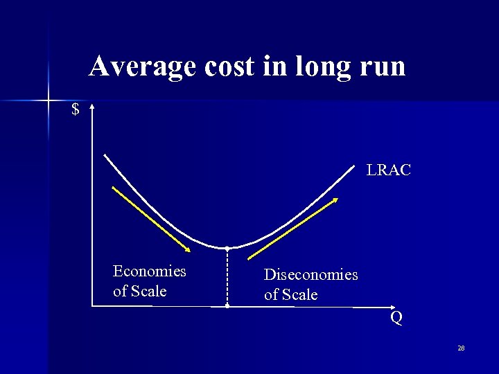Average cost in long run $ LRAC Economies of Scale Diseconomies of Scale Q 28

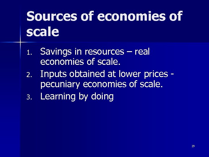Sources of economies of scale 1. 2. 3. Savings in resources – real economies of scale. Inputs obtained at lower prices - pecuniary economies of scale. Learning by doing 29

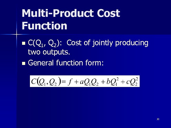Multi-Product Cost Function C(Q 1, Q 2): Cost of jointly producing two outputs. n General function form: n 30

Economies of Scope n n Cost gains made by producing two or more products together rather than separately. Example – It is cheaper for Time-Warner to produce Internet connections and Instant Messaging services jointly than separately. – Why? n Share common inputs. 31

Managerial Economics. Group A n Week Seven- Class 3 – Thursday, October 18 – 15: 10 -16: 00 – Tyndall n Next Aplia Assignment is due before 5 PM Tuesday, October 23 32

A question n The first question in the Graded MCQ for week 8 has two answer choices that are identical but worded differently. – B. the firm should use less L and more K to cost minimize. and – C. the firm should use more K and less L to cost minimize. n I was wondering if that was a typo or if those are supposed to be two of the possible answer choices. 33

My Answer You are absolutely right. Choices B and C are saying the same thing. n I changed choice B to less K and more L. n Thank you n 34

Another Question n What is an expansion path? 35

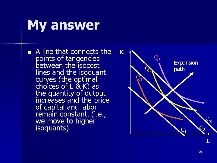My answer n A line that connects the K points of tangencies between the isocost lines and the isoquant curves (the optimal choices of L & K) as the quantity of output increases and the price of capital and labor remain constant. (i. e. , we move to higher isoquants) Q 3 Q 2 Expansion path Q 1 C 1 c 2 C 3 L 36

Cost concepts and strategic advantage 1. Firm seeks to achieve costs lower than rivals. – 2. Being the least cost operator in an industry means: – – 3. Gaining competitive advantage compared to its rivals. can charge lower prices than rival and still make profits. can charge same price and make higher profits. Sources of lower cost that rivals n economies of scope & scale 37

Cost Complementarity The marginal cost of producing good 1 declines as more of good 2 is produced: n Example: n – Cow hides and steaks MCCow hides ↓ as Q steaks↑ 38

Chapter 6 of Baye The Organization of the Firm Notes 1. You must also read the article by Michael Jensen on Blackboard. 2. The article by Gibbons (also available on Blackoard) is now recommended but not required. 39

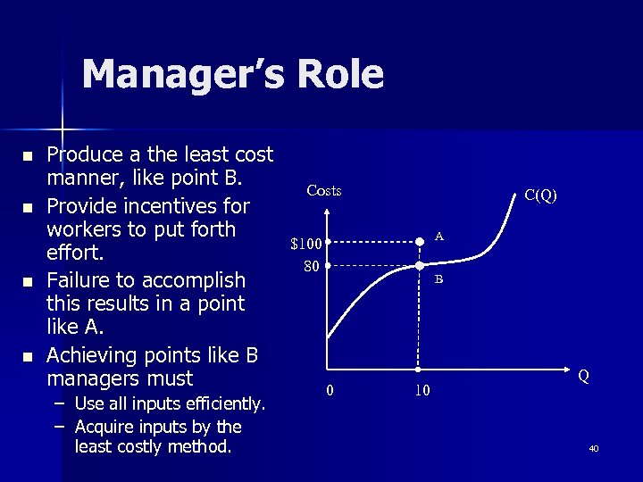Manager’s Role n n Produce a the least cost manner, like point B. Provide incentives for workers to put forth effort. Failure to accomplish this results in a point like A. Achieving points like B managers must – Use all inputs efficiently. – Acquire inputs by the least costly method. Costs C(Q) A $100 80 B 0 10 Q 40

Methods of Procuring Inputs 1. Spot Exchange – When the buyer and seller of an input meet, exchange, and then go their separate ways. – Advantages: Specialization, avoids contracting costs – Disadvantages: Possible “hold-up problem. ” 41

Here is what I saw in Brazil (spot exchange) 42

Daily workers specialize in unloading trucks 43

Methods of Procuring Inputs 2. Contracts – A legal document that creates an extended relationship between a buyer and a seller. – Example: n I have an employment contract with my university – Advantages: specialization, high productivity – Disadvantages: costly contracts, fixed cost 44

Methods of Procuring Inputs 3. Vertical Integration – A firm produces its own inputs – Example n You have a restaurant n Also produce your own pasta – Advantages: avoids contracting costs. – Disadvantages: lost specialization and may increase organizational costs. 45

Transaction Costs of acquiring an input over and above the amount paid to the input supplier. n Includes: n – Search costs. – Negotiation costs. – Other required investments or expenditures. 46

Transaction costs n Coase (1937) contrasted resource allocation in markets and in firms: – In markets, guided by price. – In firms, guided by entrepreneur co-ordinator. n n Costs of using market – transaction costs. Costs of organizing firm – governance costs. Firms are more efficient than markets because they avoid transaction costs. Compare marginal transaction and management costs. 47

Specialized Investments n Investments made to allow two parties to exchange but has little or no value outside of the exchange relationship. 48

Types of specialized investments 1. Site specificity. n You build your pasta factory near a major restaurant that buys your pasta. 2. Physical-asset specificity. n Your pasta factory uses a special machine to produce a certain type of pasta that the restaurant needs 49

Types of specialized investments 3. Dedicated assets. n The restaurant is the main customer of the pasta factory. Without that restaurant your factory will lose money. 4. Human capital. n You work for the pasta factory that uses a unique machine. If you lose that job, your skills are not useful at any other pasta factory. 50