1e779e5e2c55b92f3b298d0f43a3d896.ppt
- Количество слайдов: 49
Week 7 Sample Means & Proportions
Variability of Summary Statistics n Variability in shape of distn of sample n Variability in summary statistics n n Mean, median, st devn, upper quartile, … Summary statistics have distributions
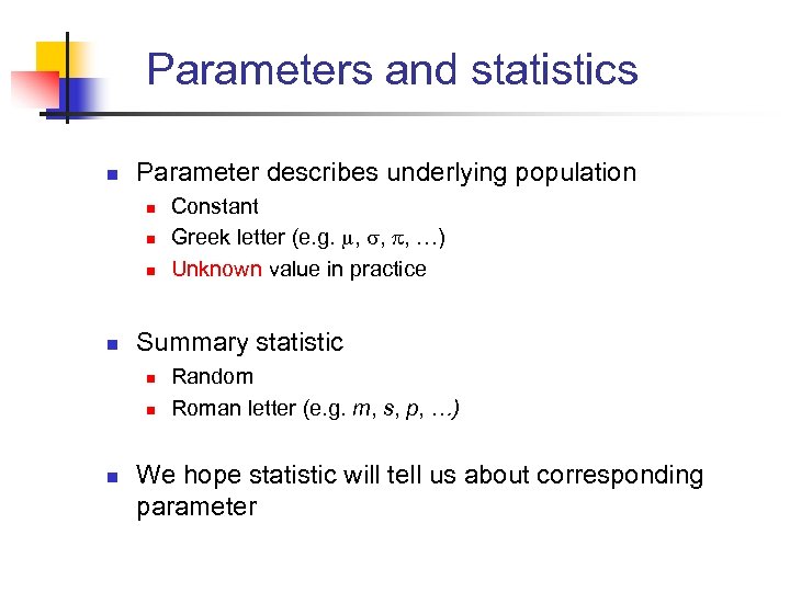
Parameters and statistics n Parameter describes underlying population n n Summary statistic n n n Constant Greek letter (e. g. , , , …) Unknown value in practice Random Roman letter (e. g. m, s, p, …) We hope statistic will tell us about corresponding parameter
Distn of sample vs Sampling distn of statistic n n n Values in a single random sample have a distribution Single sample --> single value for statistic Sample-to-sample variability of statistic is its sampling distribution.
Means n n Unknown population mean, Sample mean, X, has a distribution — its sampling distribution. Usually x ≠ A single sample mean, x, gives us information about
Sampling distribution of mean If sample size, n, increases: n n Spread of distn of sample is (approx) same. Spread of sampling distn of mean gets smaller. n n x is likely to be closer to x becomes a better estimate of
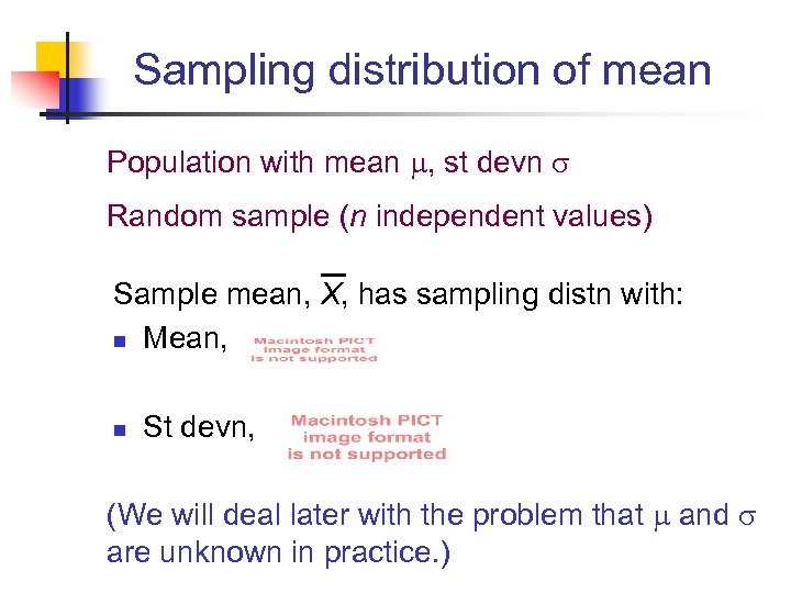
Sampling distribution of mean Population with mean , st devn Random sample (n independent values) Sample mean, X, has sampling distn with: n Mean, n St devn, (We will deal later with the problem that and are unknown in practice. )
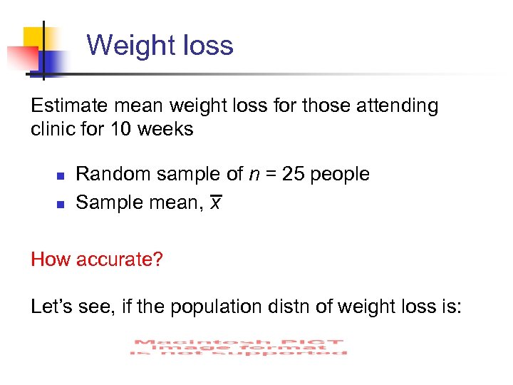
Weight loss Estimate mean weight loss for those attending clinic for 10 weeks n n Random sample of n = 25 people Sample mean, x How accurate? Let’s see, if the population distn of weight loss is:
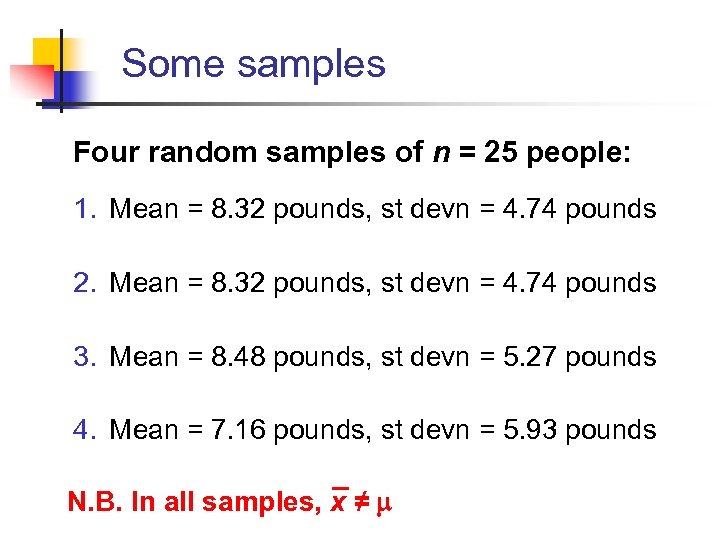
Some samples Four random samples of n = 25 people: 1. Mean = 8. 32 pounds, st devn = 4. 74 pounds 2. Mean = 8. 32 pounds, st devn = 4. 74 pounds 3. Mean = 8. 48 pounds, st devn = 5. 27 pounds 4. Mean = 7. 16 pounds, st devn = 5. 93 pounds N. B. In all samples, x ≠
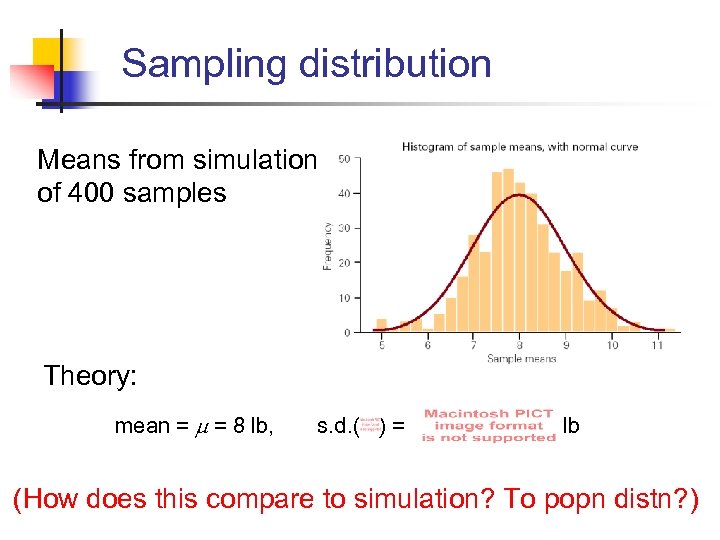
Sampling distribution Means from simulation of 400 samples Theory: mean = = 8 lb, s. d. ( ) = lb (How does this compare to simulation? To popn distn? )
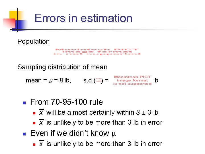
Errors in estimation Population Sampling distribution of mean = = 8 lb, s. d. ( ) = lb n From 70 -95 -100 rule n n n x will be almost certainly within 8 ± 3 lb x is unlikely to be more than 3 lb in error Even if we didn’t know n x is unlikely to be more than 3 lb in error
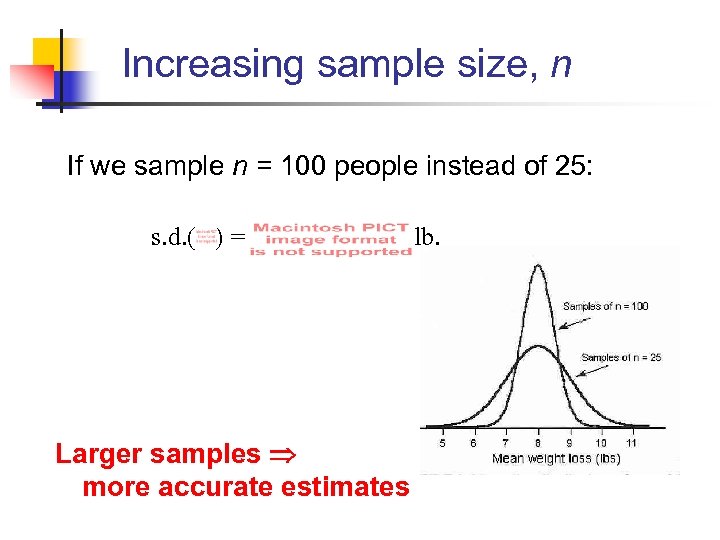
Increasing sample size, n If we sample n = 100 people instead of 25: s. d. ( ) = Larger samples more accurate estimates lb.
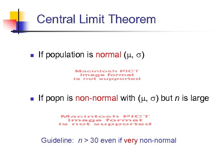
Central Limit Theorem n If population is normal ( , ) n If popn is non-normal with ( , ) but n is large Guideline: n > 30 even if very non-normal
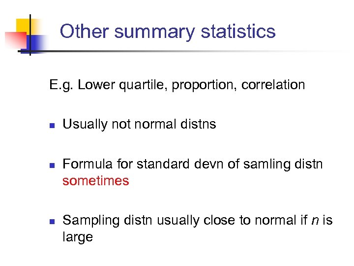
Other summary statistics E. g. Lower quartile, proportion, correlation n Usually not normal distns Formula for standard devn of samling distn sometimes Sampling distn usually close to normal if n is large
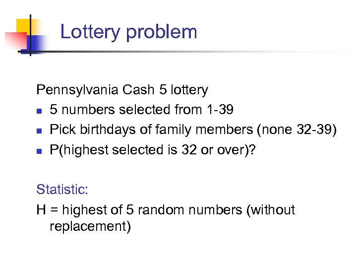
Lottery problem Pennsylvania Cash 5 lottery n 5 numbers selected from 1 -39 n Pick birthdays of family members (none 32 -39) n P(highest selected is 32 or over)? Statistic: H = highest of 5 random numbers (without replacement)
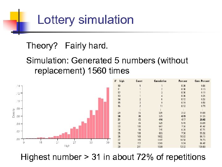
Lottery simulation Theory? Fairly hard. Simulation: Generated 5 numbers (without replacement) 1560 times Highest number > 31 in about 72% of repetitions
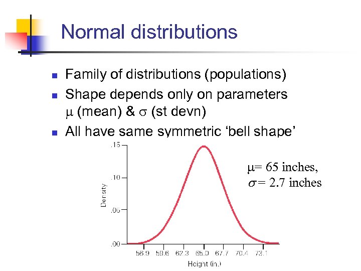
Normal distributions n n n Family of distributions (populations) Shape depends only on parameters (mean) & (st devn) All have same symmetric ‘bell shape’ = 65 inches, s = 2. 7 inches
Importance of normal distn n A reasonable model for many data sets n Transformed data often approx normal n Sample means (and many other statistics) are approx normal.
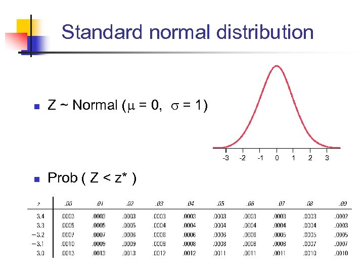
Standard normal distribution n Z ~ Normal ( = 0, = 1) -3 n Prob ( Z < z* ) -2 -1 0 1 2 3
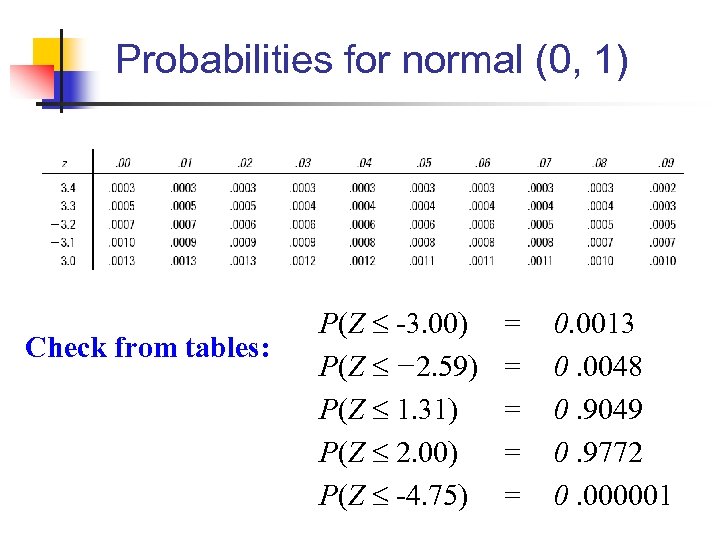
Probabilities for normal (0, 1) Check from tables: P(Z -3. 00) P(Z − 2. 59) P(Z 1. 31) P(Z 2. 00) P(Z -4. 75) = = = 0. 0013 0. 0048 0. 9049 0. 9772 0. 000001
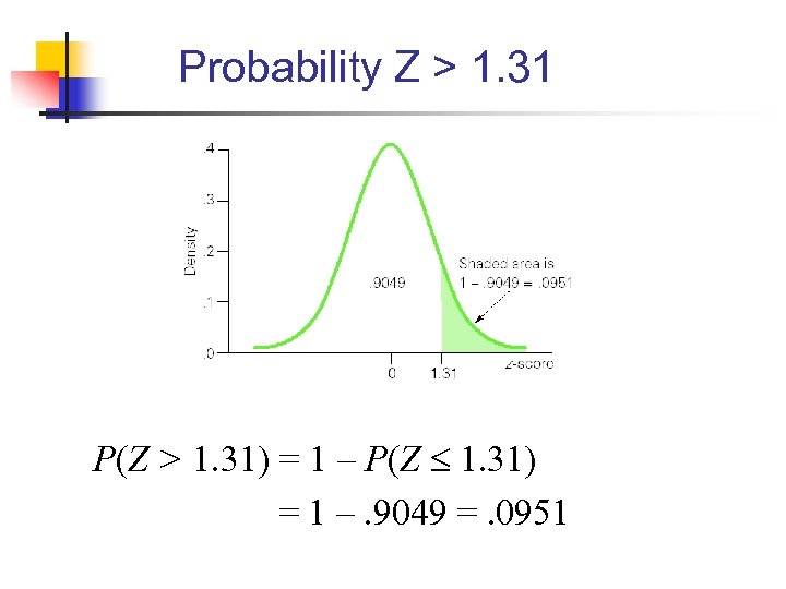
Probability Z > 1. 31 P(Z > 1. 31) = 1 – P(Z 1. 31) = 1 –. 9049 =. 0951
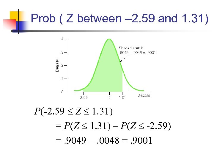
Prob ( Z between – 2. 59 and 1. 31) P(-2. 59 Z 1. 31) = P(Z 1. 31) – P(Z -2. 59) =. 9049 –. 0048 =. 9001
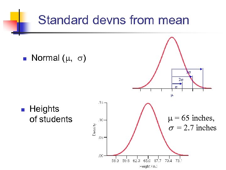
Standard devns from mean n Normal ( , ) n Heights of students = 65 inches, s = 2. 7 inches
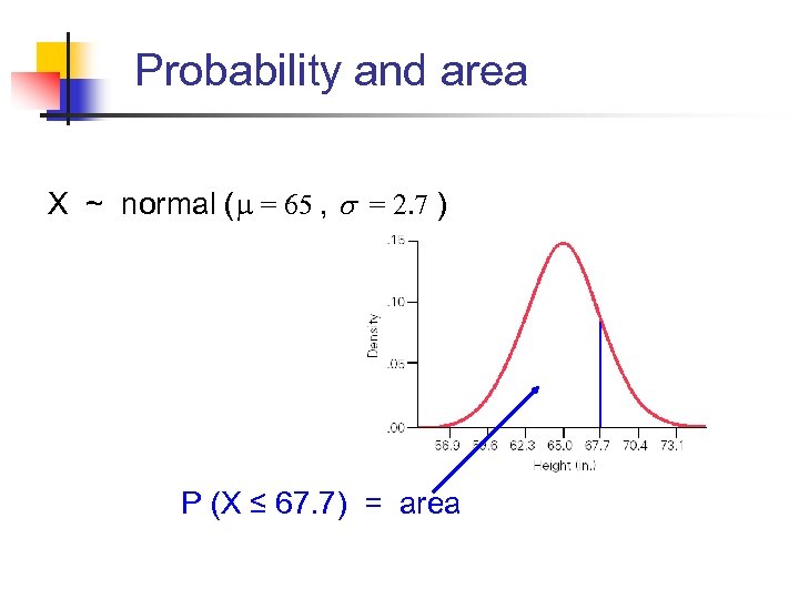
Probability and area X ~ normal ( = 65 , s = 2. 7 ) P (X ≤ 67. 7) = area
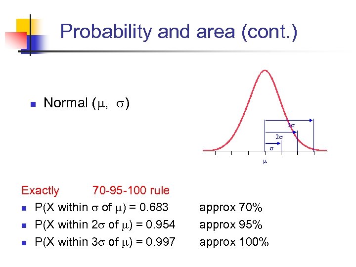
Probability and area (cont. ) n Normal ( , ) Exactly 70 -95 -100 rule n P(X within of ) = 0. 683 n P(X within 2 of ) = 0. 954 n P(X within 3 of ) = 0. 997 approx 70% approx 95% approx 100%
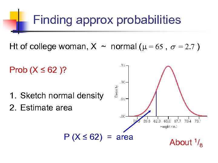
Finding approx probabilities Ht of college woman, X ~ normal ( = 65 , s = 2. 7 ) Prob (X ≤ 62 )? 1. Sketch normal density 2. Estimate area P (X ≤ 62) = area About 1/8
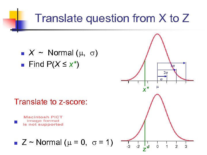
Translate question from X to Z n n X ~ Normal ( , ) Find P(X ≤ x*) x* -1 z* 0 Translate to z-score: n n Z ~ Normal ( = 0, = 1) -3 -2 1 2 3
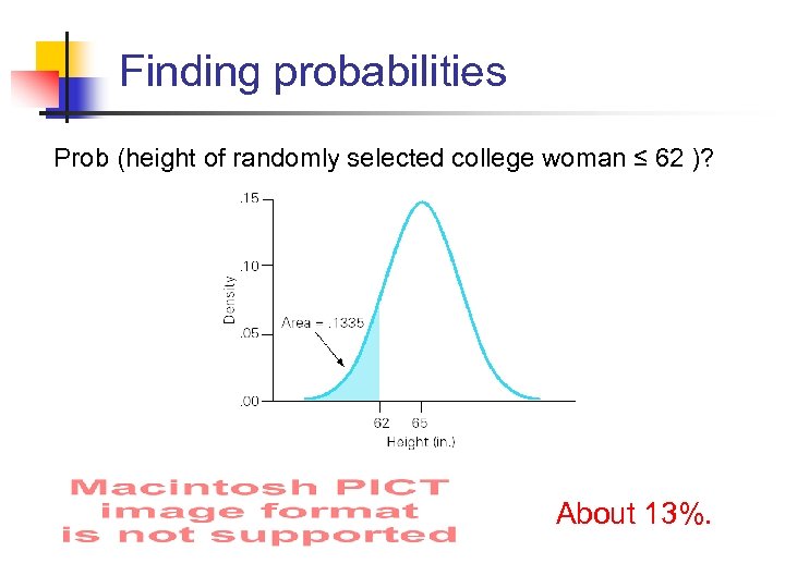
Finding probabilities Prob (height of randomly selected college woman ≤ 62 )? About 13%.
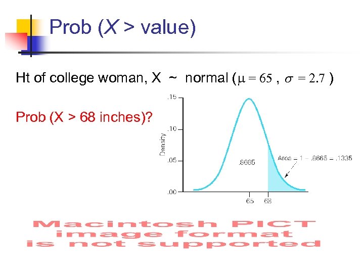
Prob (X > value) Ht of college woman, X ~ normal ( = 65 , s = 2. 7 ) Prob (X > 68 inches)?
Finding upper quartile Blood Pressures are normal with mean 120 and standard deviation 10. What is the 75 th percentile? Step 1: Solve for z-score Closest z* with area of 0. 7500 (tables) z = 0. 67 Step 2: Calculate x = z*s + x = (0. 67)(10) + 120 = 126. 7 or about 127.
Probabilities about means n Blood pressure ~ normal ( = 120, = 10) n 8 people given drug n If drug does not affect blood pressure, n Find P(average blood pressure > 130)
P ( X > 130) ? n X ~ normal ( = 120, = 10) n = 8 n n n prob = 0. 0023 n Very little chance!
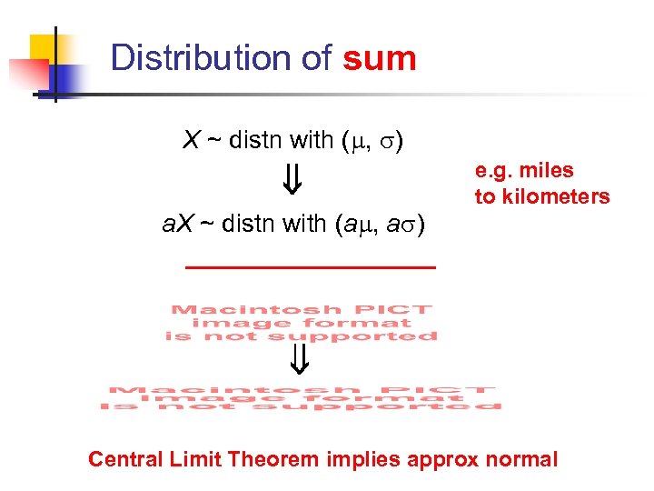
Distribution of sum X ~ distn with ( , ) e. g. miles to kilometers a. X ~ distn with (a , a ) Central Limit Theorem implies approx normal
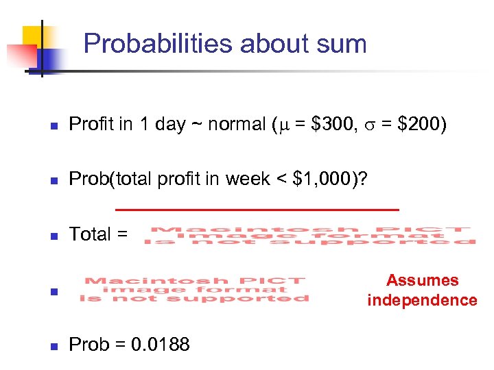
Probabilities about sum n Profit in 1 day ~ normal ( = $300, = $200) n Prob(total profit in week < $1, 000)? n Total = n n Prob = 0. 0188 Assumes independence
Categorical data n n Most important parameter is n = Prob (success) Corresponding summary statistic is n p = Proportion (success) ^ N. B. Textbook uses p and p
Number of successes n n Easiest to deal with count of successes before proportion. If… 1. n “trials” (fixed beforehand). 2. Only “success” or “failure” possible for each trial. 3. Outcomes are independent. 4. Prob (success), remains same for all trials, . • Prob (failure) is 1 – . n X = number of successes ~ binomial (n, )
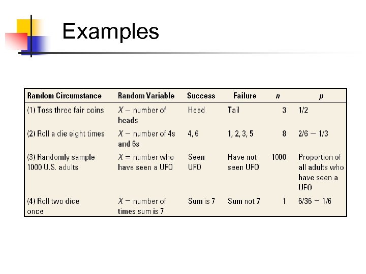
Examples
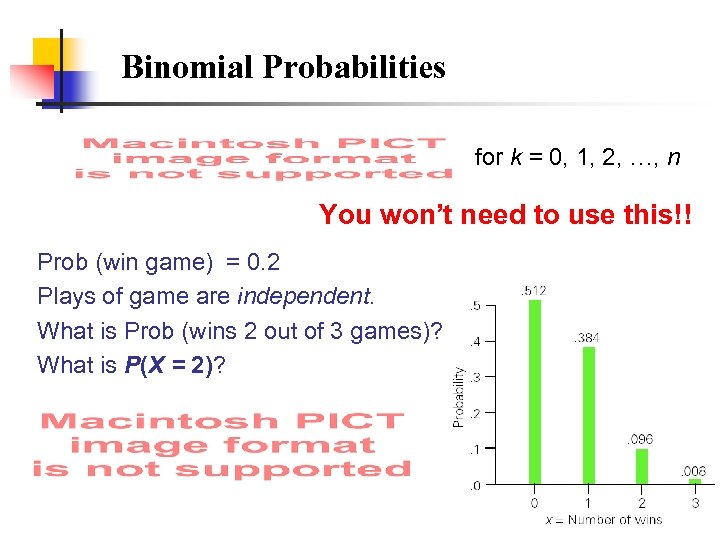
Binomial Probabilities for k = 0, 1, 2, …, n You won’t need to use this!! Prob (win game) = 0. 2 Plays of game are independent. What is Prob (wins 2 out of 3 games)? What is P(X = 2)?
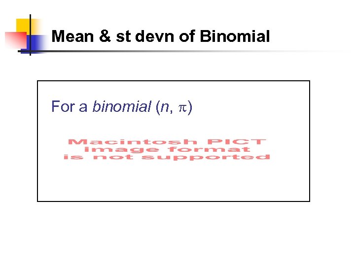
Mean & st devn of Binomial For a binomial (n, )
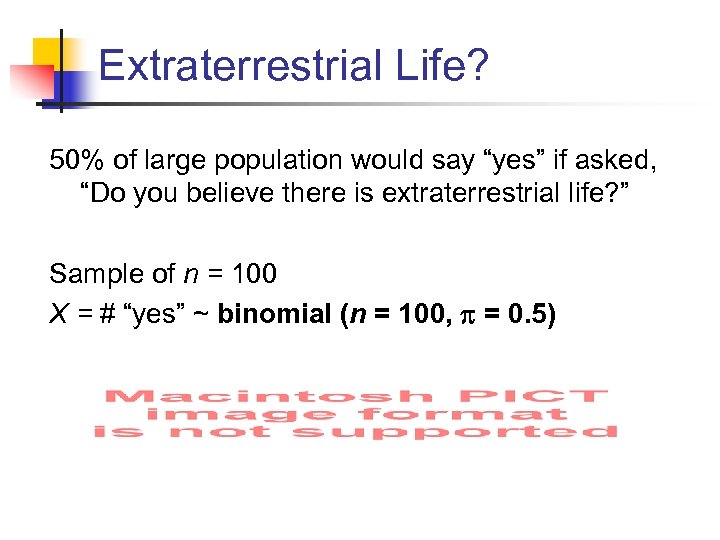
Extraterrestrial Life? 50% of large population would say “yes” if asked, “Do you believe there is extraterrestrial life? ” Sample of n = 100 X = # “yes” ~ binomial (n = 100, = 0. 5)
Extraterrestrial Life? Sample of n = 100 X = # “yes” ~ binomial (n = 100, = 0. 5) 70 -95 -100 rule of thumb for # “yes” n About 95% chance of between 40 & 60 n Almost certainly between 35 & 65
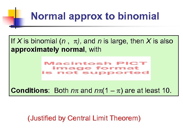
Normal approx to binomial If X is binomial (n , ), and n is large, then X is also approximately normal, with Conditions: Both n and n (1 – ) are at least 10. (Justified by Central Limit Theorem)
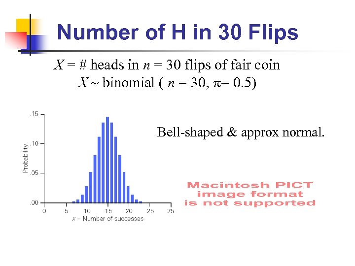
Number of H in 30 Flips X = # heads in n = 30 flips of fair coin X ~ binomial ( n = 30, = 0. 5) Bell-shaped & approx normal.
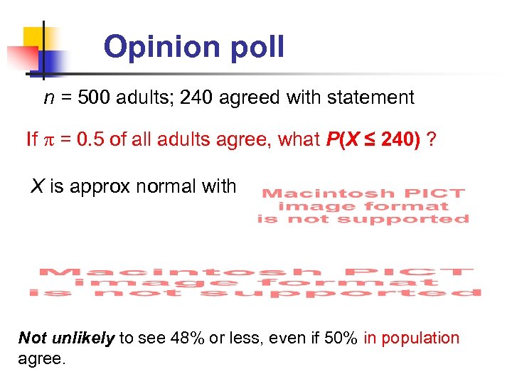
Opinion poll n = 500 adults; 240 agreed with statement If = 0. 5 of all adults agree, what P(X ≤ 240) ? X is approx normal with Not unlikely to see 48% or less, even if 50% in population agree.
Sample Proportion n n Suppose (unknown to us) 40% of a population carry the gene for a disease, ( = 0. 40). Random sample of 25 people; X = # with gene. n X ~ binomial (n = 25 , = 0. 4) p = proportion with gene
Distn of sample proportion n X ~ binomial (n , ) n Large n: p is approx normal (n ≥ 10 & n (1 – ) ≥ 10)
Examples n Election Polls: to estimate proportion who favor a candidate; units = all voters. n Television Ratings: to estimate proportion of households watching TV program; units = all households with TV. n Consumer Preferences: to estimate proportion of consumers who prefer new recipe compared with old; units = all consumers. n Testing ESP: to estimate probability a person can successfully guess which of 5 symbols on a hidden card; repeatable situation = a guess.
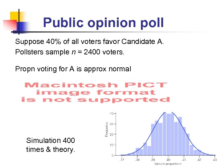
Public opinion poll Suppose 40% of all voters favor Candidate A. Pollsters sample n = 2400 voters. Propn voting for A is approx normal Simulation 400 times & theory.
Probability from normal approx If 40% of voters favor Candidate A, and n = 2400 sampled Sample proportion, p, is almost certain to be between 0. 37 and 0. 43 Prob 0. 95 of p being between 0. 38 and 0. 42
1e779e5e2c55b92f3b298d0f43a3d896.ppt