Watershed and Stream Network Delineation

Watershed and Stream Network Delineation • • • Grid digital elevation models (DEM) Eight Direction Pour Point Model Contributing Area Pits and Pit Removal Channel Network Delineation Channel Network Geomorphology

Elevation Surface — the ground surface elevation at each point Digital Elevation Model — A digital representation of an elevation surface. Examples include a (square) digital elevation grid, triangular irregular network, set of digital line graph contours or random points.

Digital Elevation Grid — a grid of cells (square or rectangular) in some coordinate system having land surface elevation as the value stored in each cell. Square Digital Elevation Grid — a common special case of the digital elevation grid

DEM Data Sources • 30 m DEMs from 1: 24, 000 scale maps • 3" (100 m) DEMs from 1: 250, 000 scale maps • 15" DEM for the US resampled from 3” Dem • 30" DEM of the earth (GTOPO 30)

30 m DEMs • Best resolution standardized data source available for the US • Coverage of the country is incomplete • Data by 7. 5’ map sheets in UTM projection • Link for US (USGS EROS Data Center) http: //edcwww. cr. usgs. gov/doc/edchome/ndcdb. html

3” DEMs • Derived by US Defence Mapping Agency, available from USGS for the whole US • Data in geographic coordinates by 1; 250, 000 map sheet names (1ºx 1º) cells in (1ºx 2º) maps • Needs to be projected to planar coordinates • Link for US (USGS EROS Data Center) http: //edcwww. cr. usgs. gov/doc/edchome/ndcdb. html

Coverage of 30 m and 3" DEMs 3" (100 m) DEM 1º 30 m DEM 7. 5´ 1º

30 m Cell Size 100 m

A Case Study of Hog Pen Creek Hog Pen Ck 4 km

Watershed Delineation by Hand Digitizing 20 ft contour Watershed divide 100 ft contour Stream Center Line Drainage direction Outlet

30 Meter Mesh Standard for 1: 24, 000 Scale Maps

DEM Elevations 720 Contours 740 720 700 680

Direction of Steepest Descent 30 30 67 49 67 56 49 52 48 37 58 Slope: 56 55 22 58 55 22

Eight Direction Pour Point Model D 8 4 3 1 5 6 2 7 8

Grid Network

Contributing Area Grid 1 1 4 1 1 1 1 3 12 2 3 6 1 1 1 3 1 1 4 3 3 1 2 1 1 1 1 1 2 16 1 1 3 6 25 2 16 25 2

Contributing Area > 10 Cell Threshold 1 1 1 4 3 3 1 12 1 1 2 16 1 1 3 6 25 2

Watershed Draining to This Outlet

Watershed and Drainage Paths Delineated from 30 m DEM Automated method is more consistent than hand delineation

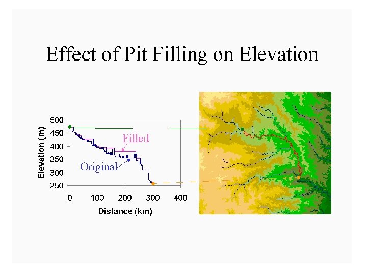
Filling in the Pits • DEM creation results in artificial pits in the landscape • A pit is a set of one or more cells which has no downstream cells around it • Unless these pits are filled they become sinks and isolate portions of the watershed • Pit filling is first thing done with a DEM

How to decide on support area threshold ? AREA 2 3 AREA 1 12

Streams from 1: 250, 000 blue lines

100 grid cell constant support area threshold stream delineation

200 grid cell constant support area based stream delineation

Examples of differently textured topography Badlands in Death Valley. from Easterbrook, 1993, p 140. Coos Bay, Oregon Coast Ra from W. E. Dietrich

Canyon Creek, Trinity Alps, Northern California. Photo D K Hagans

Gently Sloping Convex Landscape From W. E. Dietrich

Mancos Shale badlands, Utah. From Howard, 1994.

Topographic Texture and Drainage Density Driftwood, PA Same scale, 20 m contour interval Sunland, CA

Contrasting Interpretations “landscape dissection into distinct valleys is limited by a threshold of channelization that sets a finite scale to the landscape. ” (Montgomery and Dietrich, 1992, Science, vol. 255 p. 826. ) “any definition of a finite channel network is arbitrary, and entirely scale dependent. ” (Band, 1993, in “Channel Network Hydrology”, edited by Beven and Kirkby, p 15. )

Suggestion: One contributing area threshold does not fit all watersheds. Lets look at some geomorphology. • Drainage Density • Horton’s Laws • Stream Drops • Slope-Area properties • Hack’s Law

Drainage Density • Dd = L/A • Hillslope length 1/2 Dd B B Hillslope length = B L A = 2 B L Dd = L/A = 1/2 B B= 1/2 Dd

Drainage Density for Different Support Area Thresholds EPA Reach Files 100 grid cell threshold 1000 grid cell threshold

Drainage Density Versus Contributing Area Threshold

Hortons Laws: Strahler system for stream ordering 1 1 2 2 1 3 1 1 2 1 1 1 1

Bifurcation Ratio

Length Ratio

Area Ratio

Slope Ratio

Constant Stream Drops

Slope-Area scaling Data from Reynolds Creek 30 m DEM, 50 grid cell threshold, points, individual links, big dots, bins of size 100

Hack’s Law

Suggestion: Map channel networks from the DEM at the finest resolution consistent with observed channel network geomorphology ‘laws’. • Break in slope versus contributing area scaling • Break in Constant stream drop property • Physical basis in the form instability theory of Smith and Bretherton (1972), see Tarboton et al. 1992

Constant Support Area Threshold

Channel network delineation, other options 4 2 3 5 6 1 7 8 Accumulation Area Grid Order 1 1 1 4 3 3 1 1 2 2 2 1 12 1 1 3 1 1 2 16 1 1 3 6 25 2 1 2 2 3 1

Grid network pruned to order 4 stream delineation

Curvature based stream delineation

Local Curvature Computation (Peuker and Douglas, 1975, Comput. Graphics Image Proc. 4: 375) 43 48 48 51 51 56 41 47 47 54 54 58

Contributing area of upwards curved grid cells only

Upward Curved Contributing Area Threshold

• Grid Processing TARDEM Components • [streamtogrid] – tdprepro • Flood • D 8 • [Dinf] • Aread 8 • [Areadinf] • Gridnet • Channel Network and Subwatershed delineation – Netsetup – Subbasinsetup • Conversion to Arc Coverage (export *. E 00) – Arclinks – Arcstreams • Analysis – Linkan – Streaman – Asfgrid

Summary Concepts • Topographic maps are the traditional way of representing land surface terrain and streams • Watersheds can be hand-delineated from these maps • DEM’s of equivalent accuracy are now available for most map series in the US

Summary Concepts (2) • DEM cell elevation is at the cell center • eight direction pour point model leads to flow direction and contributing area grids • A simple stream network is defined as cells whose contributing area exceeds a threshold

Summary Concepts (3) • Channel networks obey Hortons laws. • Use consistency with Hortons laws to adapt support area threshold and drainage density to the natural texture of the topography. • Use curvature based methods to allow channel network drainage density to be spatially variable to adapt to variable topographic texture.