Water Resources Systems Modeling Techniques Prof V Jothiprakash

Water Resources Systems Modeling Techniques Prof. V. Jothiprakash Assistant Professor Department of Civil Engineering Indian Institute of Technology Bombay Powai, Mumbai 400 076 vprakash@civil. iitb. ac. in 1

Introduction • Water – Crucial element for human survival – Key element in the socio-economic development of a country • Demand – Increasing • Extensive and intensive agriculture • Power production • Municipal and industrial use (urbanization and industrialization) 2

Contd… – Availability • Constant over a period of time • Spatial and temporal variations – To over come this variations and to meet the demands » Judicial use is needed » Effective and efficient utilization is also needed • Large, medium and small reservoirs – Need to be operated to optimal condition » The best possible manner – Requires systematic study 3

SWOT analysis of Water Resources • Strength – India is gifted with large number of rivers – 400 x 1010 m 3 of water available • Weakness – Spatial and temporal distribution • • Rainfall 11, 500 mm at Cherrapunji 215 mm at Jaisalamer 69 x 1010 m 3 is utilizable form Storage insufficient to meet the demand Monsoon failure or excess rainfall in one monsoon 4

Contd… – Reservoirs • • • Improperation No single algorithm available to solve WR problem Topography does not allow construction of very large dams Improper understanding of the hydrological phenomena Complex interaction between human and nature 5

Contd… • Opportunities – To store them in small reservoirs – To operate the reservoirs optimally • To allocate water to various users • To maximize the economic return – – Augment the sources On form developmental works Reuse and recycling Desalinization 6

Contd… • Threats – – Large spatial and temporal variations Demand is ever increasing Sociological problems Implementation of best polices But in INDIA many reservoirs need optimal operating polices – Systematic study is needed 7

Solving the problems-really we solve it? • Real life problems are solved – – By developing theoretical equations My models Some time based on experience Most of the time SHM – Some How Managed • In Engineering – Four Generations-in solutions • • Empirical methods/Experiments Analytical Equations Numerical schemes Systems approach Data Driven methods Soft computing techniques 8

Empirical methods/ Model Experiments • Based on the observed data and their statistical correlations – conventional models • Conducting experimental works and relating it to the real world problems • Started long back, now againing importance by introduction of new ANN models 9

Engineering problem solving Generations • Numerical Schemes – Finite Difference Scheme – Finite Element Scheme • These are possible only when equations are possible to develop and solve (high order differential equations solved using computers) • Data driven methods New yet to be widely accepted 10

MODELS Characteristic representation of the prototype • Iconic models • Physical models • Analogue models • Mathematical models – Optimization (prescriptive models) • Best solution – Simulation (descriptive models) • Answers “what if” conditions 11

Why we need model studies? ? ? USES of MODEL STUDIES • To study the behaviour of the prototype • To study the impact of the prototype • To study the effect of the variation in the parameters • To solve the real world problems • Prototype are costlier and time consuming-once constructed they cannot be changed? • Thus before going in for prototype a model study will be carried out • It is very important in Water Resources – Dam design and analysis, flow condition over a spill way, dam break analysis, operation of reservoirs, planning of canal management etc…. 12

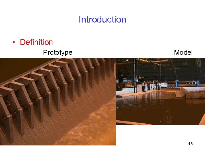Introduction • Definition – Prototype - Model 13

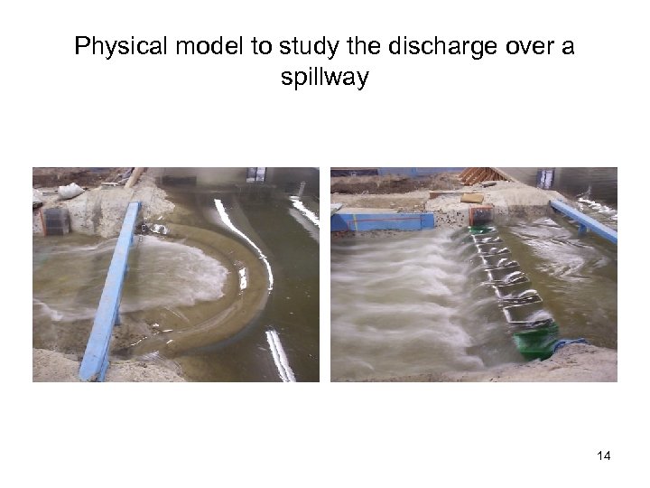Physical model to study the discharge over a spillway 14

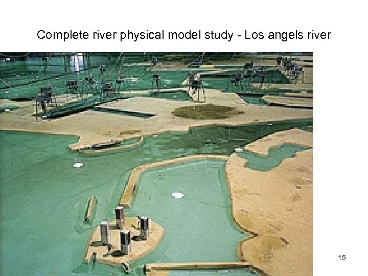Complete river physical model study - Los angels river 15

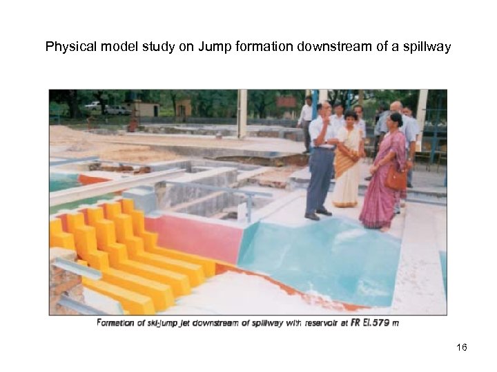Physical model study on Jump formation downstream of a spillway 16

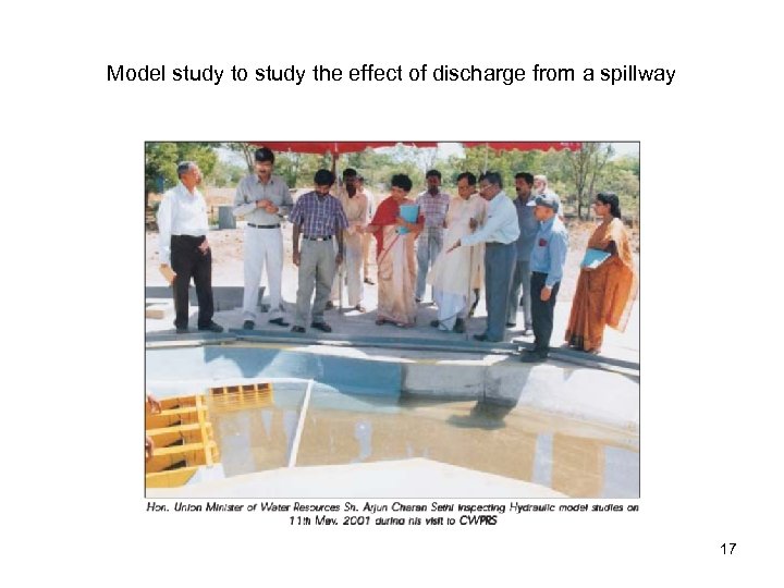Model study to study the effect of discharge from a spillway 17

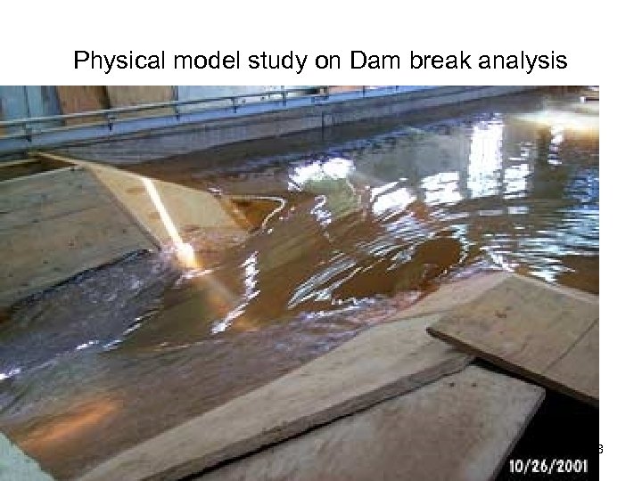Physical model study on Dam break analysis 18

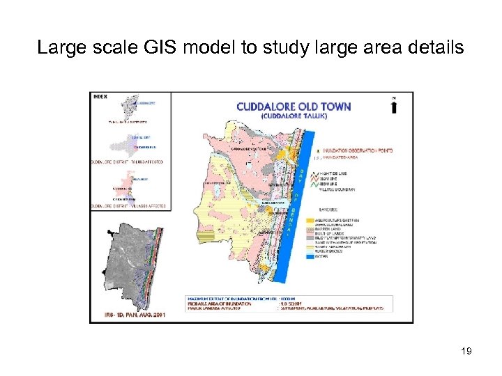Large scale GIS model to study large area details 19

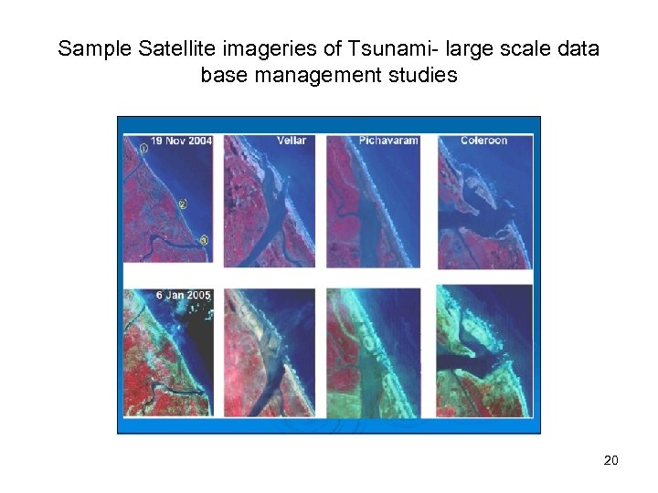Sample Satellite imageries of Tsunami- large scale data base management studies 20

Systems Approach Mathematical Modeling 21

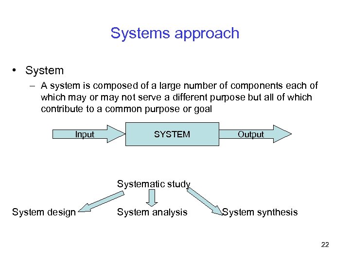Systems approach • System – A system is composed of a large number of components each of which may or may not serve a different purpose but all of which contribute to a common purpose or goal Input SYSTEM Output Systematic study System design System analysis System synthesis 22

Why we need systems approach? 1. System is large and complex 2. System should involve / necessitate knowledge from many disciplines 3. The objective need to be quantified in mathematical terms (or logical terms) 4. One or more variables involve uncertainty 5. The problem has many alternative solutions 23

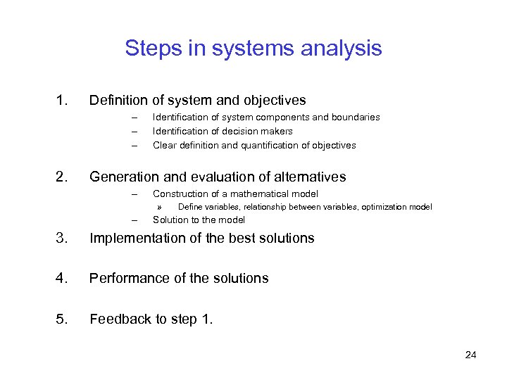Steps in systems analysis 1. Definition of system and objectives – – – 2. Identification of system components and boundaries Identification of decision makers Clear definition and quantification of objectives Generation and evaluation of alternatives – Construction of a mathematical model » – Define variables, relationship between variables, optimization model Solution to the model 3. Implementation of the best solutions 4. Performance of the solutions 5. Feedback to step 1. 24

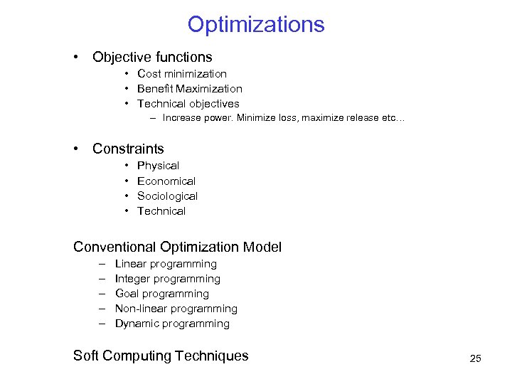Optimizations • Objective functions • Cost minimization • Benefit Maximization • Technical objectives – Increase power. Minimize loss, maximize release etc… • Constraints • • Physical Economical Sociological Technical Conventional Optimization Model – – – Linear programming Integer programming Goal programming Non-linear programming Dynamic programming Soft Computing Techniques 25

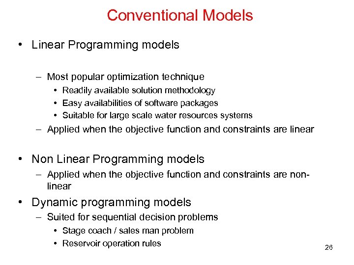Conventional Models • Linear Programming models – Most popular optimization technique • Readily available solution methodology • Easy availabilities of software packages • Suitable for large scale water resources systems – Applied when the objective function and constraints are linear • Non Linear Programming models – Applied when the objective function and constraints are nonlinear • Dynamic programming models – Suited for sequential decision problems • Stage coach / sales man problem • Reservoir operation rules 26

Simulation • Used for the evaluation of the performance of water resources systems • Can answer “what if condition” • Now a days mostly used along with optimizations 27

Soft Computing Techniques 28

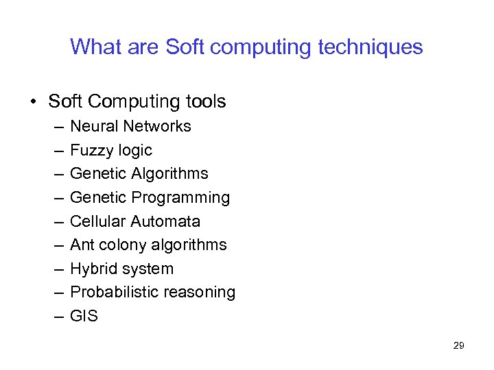What are Soft computing techniques • Soft Computing tools – – – – – Neural Networks Fuzzy logic Genetic Algorithms Genetic Programming Cellular Automata Ant colony algorithms Hybrid system Probabilistic reasoning GIS 29

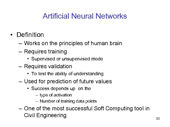Artificial Neural Networks • Definition – Works on the principles of human brain – Requires training • Supervised or unsupervised mode – Requires validation • To test the ability of understanding – Used for prediction of future values • Success depends up on the – type of activation – Number of training data points – One of the most successful Soft Computing tool in Civil Engineering 30

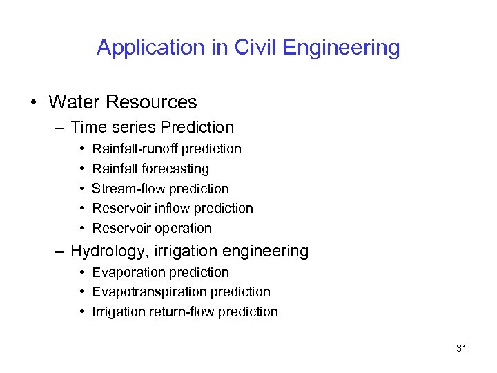Application in Civil Engineering • Water Resources – Time series Prediction • • • Rainfall-runoff prediction Rainfall forecasting Stream-flow prediction Reservoir inflow prediction Reservoir operation – Hydrology, irrigation engineering • Evaporation prediction • Evapotranspiration prediction • Irrigation return-flow prediction 31

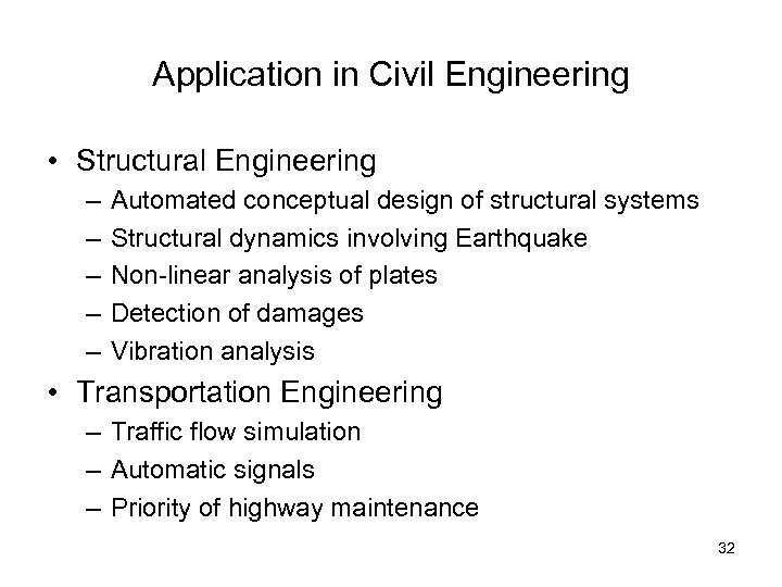Application in Civil Engineering • Structural Engineering – – – Automated conceptual design of structural systems Structural dynamics involving Earthquake Non-linear analysis of plates Detection of damages Vibration analysis • Transportation Engineering – Traffic flow simulation – Automatic signals – Priority of highway maintenance 32

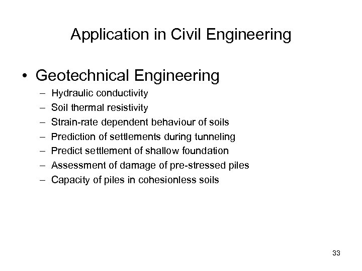Application in Civil Engineering • Geotechnical Engineering – – – – Hydraulic conductivity Soil thermal resistivity Strain-rate dependent behaviour of soils Prediction of settlements during tunneling Predict settlement of shallow foundation Assessment of damage of pre-stressed piles Capacity of piles in cohesionless soils 33

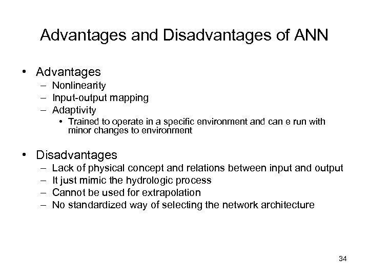Advantages and Disadvantages of ANN • Advantages – Nonlinearity – Input-output mapping – Adaptivity • Trained to operate in a specific environment and can e run with minor changes to environment • Disadvantages – – Lack of physical concept and relations between input and output It just mimic the hydrologic process Cannot be used for extrapolation No standardized way of selecting the network architecture 34

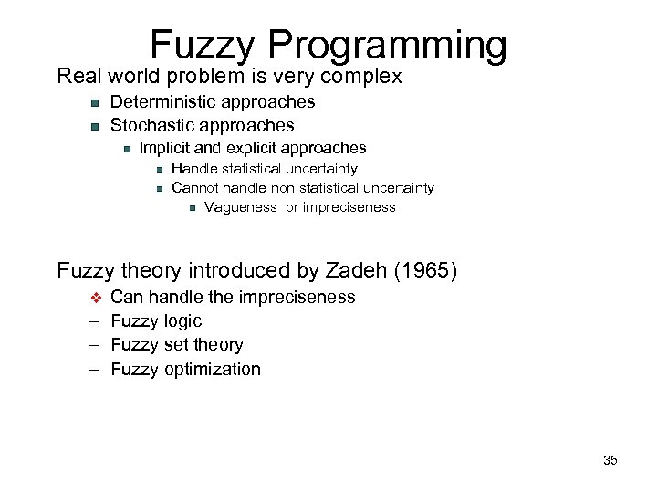Fuzzy Programming Real world problem is very complex Deterministic approaches Stochastic approaches Implicit and explicit approaches Handle statistical uncertainty Cannot handle non statistical uncertainty Vagueness or impreciseness Fuzzy theory introduced by Zadeh (1965) Can handle the impreciseness – Fuzzy logic – Fuzzy set theory – Fuzzy optimization v 35

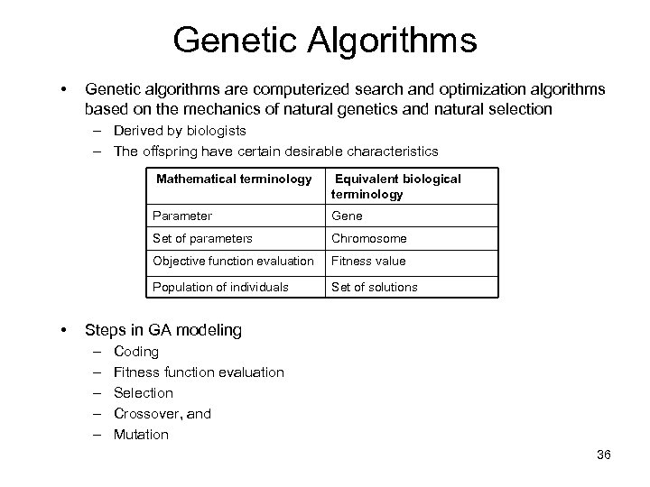Genetic Algorithms • Genetic algorithms are computerized search and optimization algorithms based on the mechanics of natural genetics and natural selection – Derived by biologists – The offspring have certain desirable characteristics Mathematical terminology Parameter Gene Set of parameters Chromosome Objective function evaluation Fitness value Population of individuals • Equivalent biological terminology Set of solutions Steps in GA modeling – – – Coding Fitness function evaluation Selection Crossover, and Mutation 36

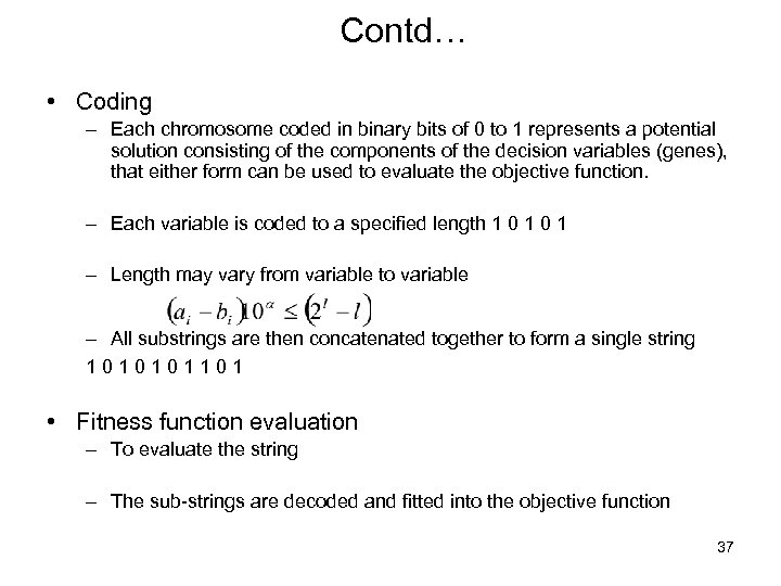Contd… • Coding – Each chromosome coded in binary bits of 0 to 1 represents a potential solution consisting of the components of the decision variables (genes), that either form can be used to evaluate the objective function. – Each variable is coded to a specified length 1 0 1 – Length may vary from variable to variable – All substrings are then concatenated together to form a single string 1010101101 • Fitness function evaluation – To evaluate the string – The sub-strings are decoded and fitted into the objective function 37

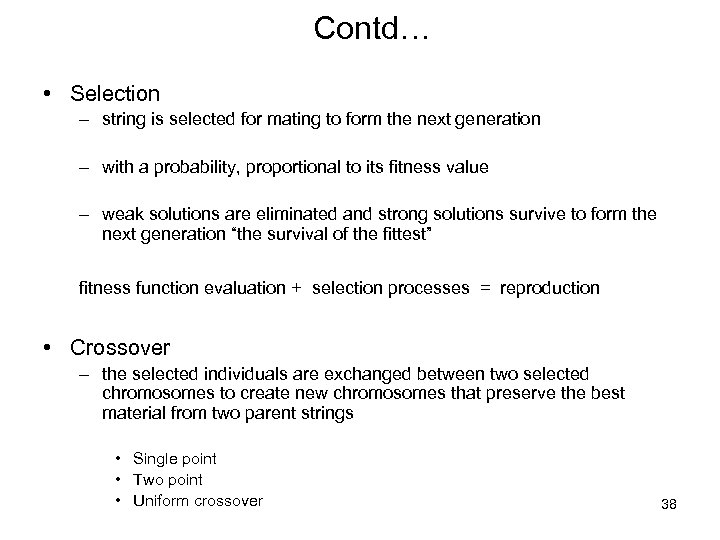Contd… • Selection – string is selected for mating to form the next generation – with a probability, proportional to its fitness value – weak solutions are eliminated and strong solutions survive to form the next generation “the survival of the fittest” fitness function evaluation + selection processes = reproduction • Crossover – the selected individuals are exchanged between two selected chromosomes to create new chromosomes that preserve the best material from two parent strings • Single point • Two point • Uniform crossover 38

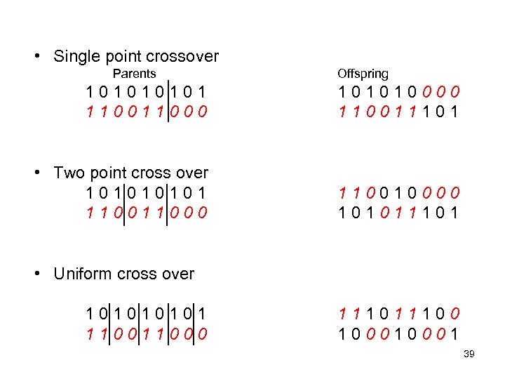• Single point crossover Parents Offspring 10101 1 1 0 0 0 1 0 1 0 0 1 1 1 0 1 • Two point cross over 10101 1 1 0 0 0 0 1 0 1 1 1 0 1 • Uniform cross over 10101 1 1 0 0 0 1 1 1 0 0 0 1 39

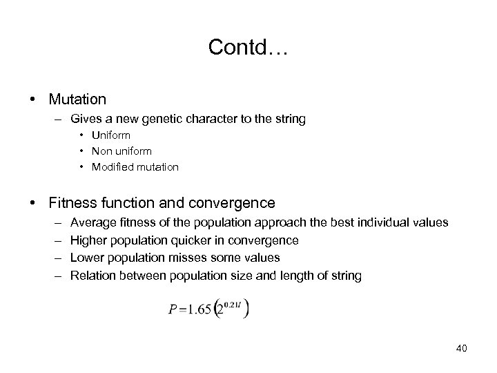Contd… • Mutation – Gives a new genetic character to the string • Uniform • Non uniform • Modified mutation • Fitness function and convergence – – Average fitness of the population approach the best individual values Higher population quicker in convergence Lower population misses some values Relation between population size and length of string 40

Application of GA in water resources • Pipe network – Design of networks, and analysis • Ground water management problems – Quantity and quality management models • Reservoir operation – – Single purpose single reservoir Multi-reservoir systems Multi-purpose multi-reservoir systems 41

Advantages of GA model 1. The GA typically uses a coding of the decision variable set, not the decision variable itself 2. The GA searches from a population of decision variable sets, not a single decision variable set 3. The GA uses the objective function itself not the derivative information 4. The GA algorithm uses probabilistic (not deterministic) search rules 5. GA takes care of stochasticity also 6. GA does not requires discretization of state variables 7. GA does not requires transition probabilities 8. GA does not have curse of dimensionality problems 9. GA models results in optimal or near optimal solutions 42

Disadvantages of GA model 1. Cannot handle large number of constraints like LP models 2. Computationally difficult to provide very long string length with binary coding - To some extent overcome by hexagonal coding 3. Every iteration need objective function evaluation 4. Difficult to handle mutation Still GA model provide better solutions than the conventional optimization techniques in developing reservoir operating rules 43

Application case study – 1 Artificial Neural Network model to predict inflow into a reservoir 44

Inflow into a reservoir Most important input variable in water resources planning and management Considered as Deterministic variable Probabilistic variable Stochastic variable Fuzzy variable Historical data or Generated data 45

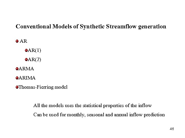Conventional Models of Synthetic Streamflow generation AR AR(1) AR(2) ARMA ARIMA Thomas-Fierring model All the models uses the statistical properties of the inflow Can be used for monthly, seasonal and annual inflow prediction 46

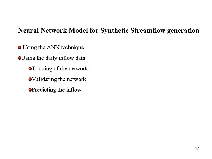Neural Network Model for Synthetic Streamflow generation Using the ANN technique Using the daily inflow data Training of the network Validating the network Predicting the inflow 47

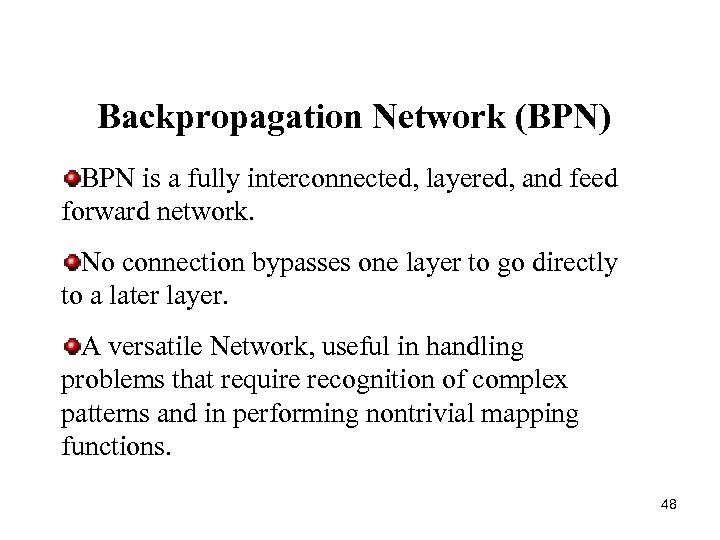Backpropagation Network (BPN) BPN is a fully interconnected, layered, and feed forward network. No connection bypasses one layer to go directly to a later layer. A versatile Network, useful in handling problems that require recognition of complex patterns and in performing nontrivial mapping functions. 48

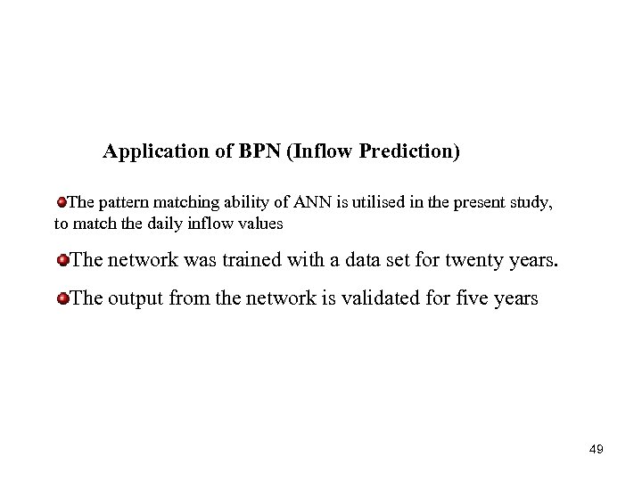Application of BPN (Inflow Prediction) The pattern matching ability of ANN is utilised in the present study, to match the daily inflow values The network was trained with a data set for twenty years. The output from the network is validated for five years 49

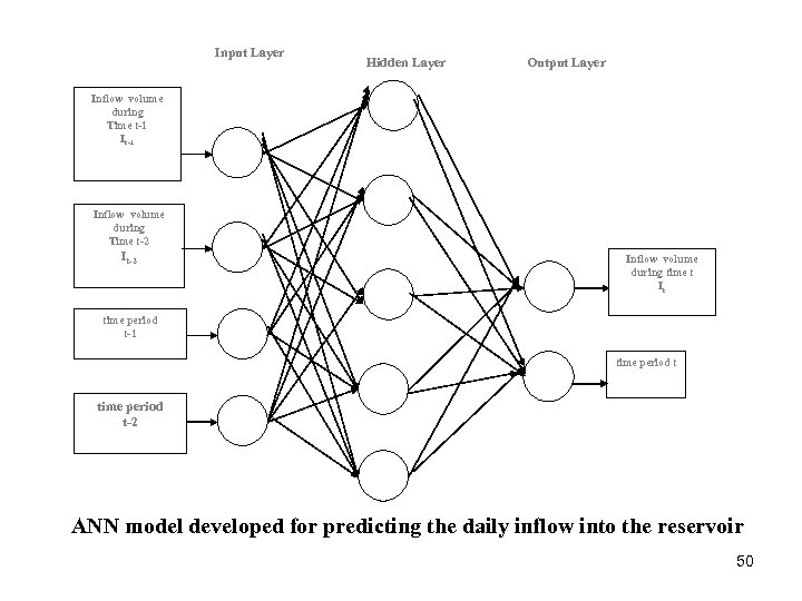Input Layer Hidden Layer Output Layer Inflow volume during Time t-1 Inflow volume during Time t-2 Inflow volume during time t It time period t-1 time period t-2 ANN model developed for predicting the daily inflow into the reservoir 50

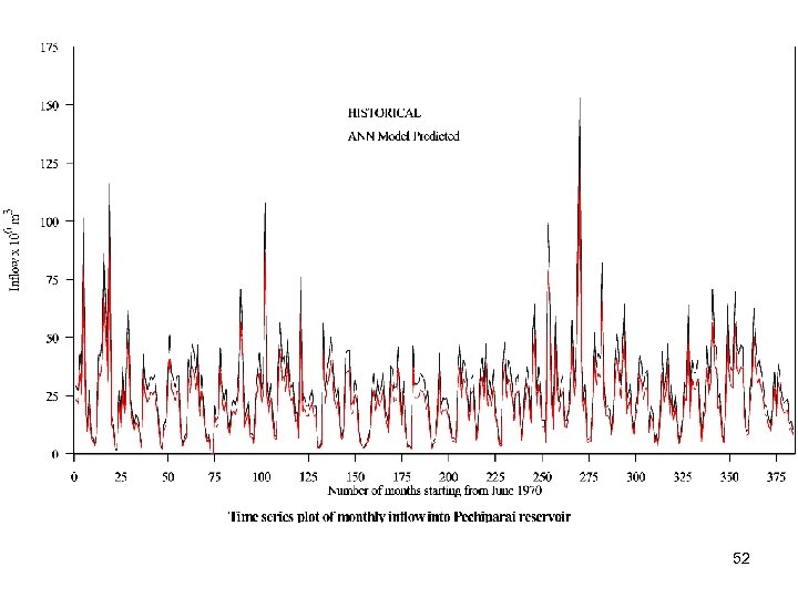
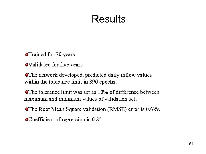Results Trained for 20 years Validated for five years The network developed, predicted daily inflow values within the tolerance limit in 390 epochs. The tolerance limit was set as 10% of difference between maximum and minimum values of validation set. The Root Mean Square validation (RMSE) error is 0. 629. Coefficient of regression is 0. 85 51

52

Application case study – 2 Application of Artificial. Neural Network to predict Reference crop evapotranspiration 53

Reference crop evapotranspiration (Ref-ETr) Estimation of Ref-ETr is indispensable for an effective management of water resources Numerous methods varying from simple empirical equation to complex methods are available for its estimation. 54

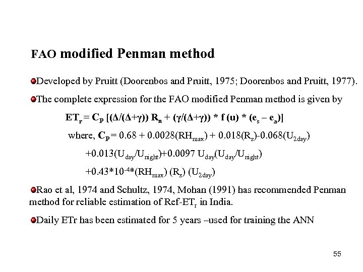FAO modified Penman method Developed by Pruitt (Doorenbos and Pruitt, 1975; Doorenbos and Pruitt, 1977). The complete expression for the FAO modified Penman method is given by ETr = CP [(Δ/(Δ+γ)) Rn + (γ/(Δ+γ)) * f (u) * (es – ea)] where, CP = 0. 68 + 0. 0028(RHmax) + 0. 018(Rs)-0. 068(U 2 day) +0. 013(Uday/Unight)+0. 0097 Uday(Uday/Unight) +0. 43*10 -4*(RHmax) (Rs) (U 2 day) Rao et al, 1974 and Schultz, 1974, Mohan (1991) has recommended Penman method for reliable estimation of Ref-ETr in India. Daily ETr has been estimated for 5 years –used for training the ANN 55

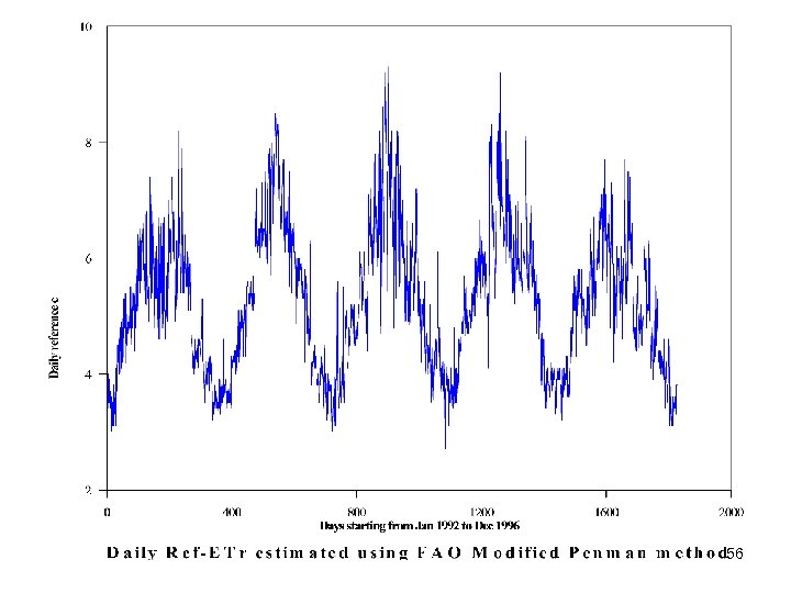56

Application of BPN (The Ref-ETr network) The pattern matching ability of ANN is utilised in the present study, to match the Ref-ETr values to its four vital parameters namely, relative humidity, maximum and minimum temperature and wind speed. The network was trained with a data set for five years. 57

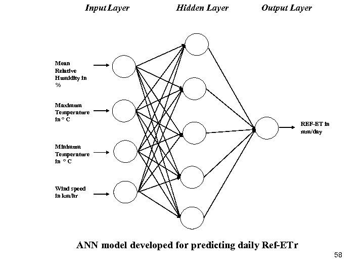Input Layer Hidden Layer Output Layer Mean Relative Humidity in % Maximum Temperature in ° C REF-ET in mm/day Minimum Temperature in ° C Wind speed in km/hr ANN model developed for predicting daily Ref-ETr 58

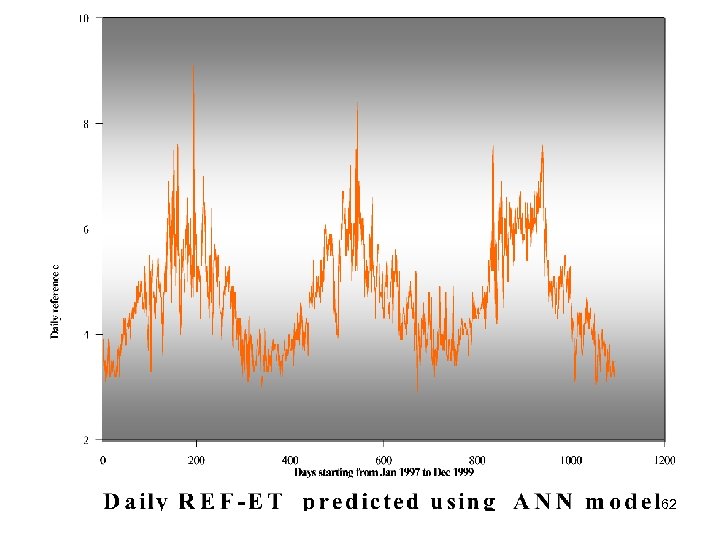
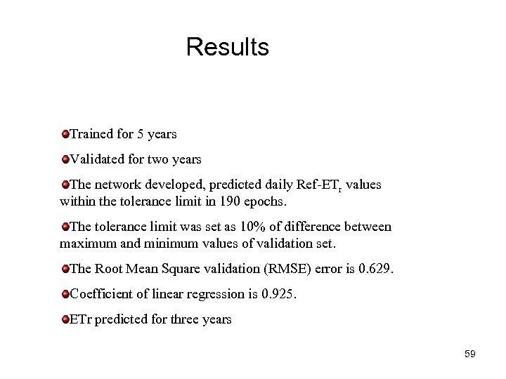Results Trained for 5 years Validated for two years The network developed, predicted daily Ref-ETr values within the tolerance limit in 190 epochs. The tolerance limit was set as 10% of difference between maximum and minimum values of validation set. The Root Mean Square validation (RMSE) error is 0. 629. Coefficient of linear regression is 0. 925. ETr predicted for three years 59

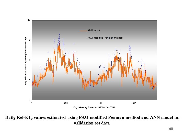Daily Ref-ETr values estimated using FAO modified Penman method and ANN model for validation set data 60

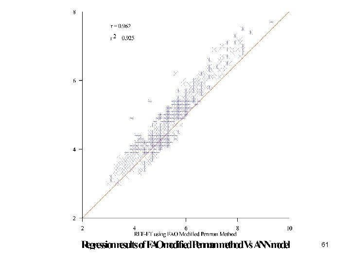61

62

Application case study – 3 Fuzzy Linear Programming model to derive optimal crop plans in a command area 63

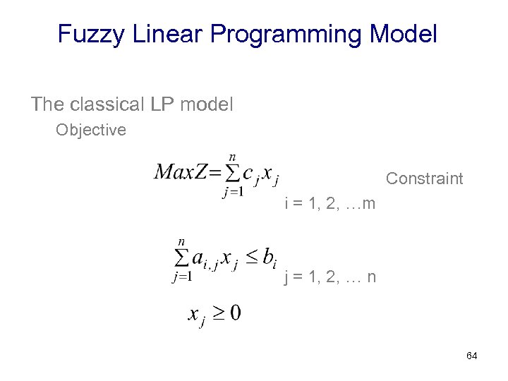Fuzzy Linear Programming Model The classical LP model Objective Constraint i = 1, 2, …m j = 1, 2, … n 64

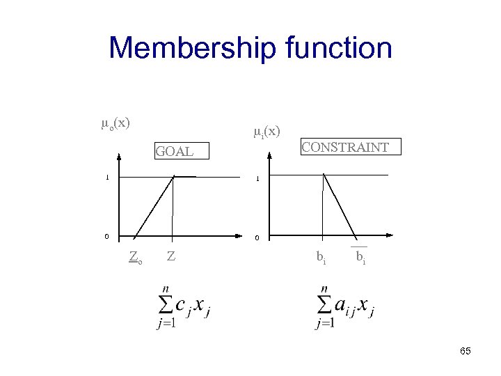Membership function o(x) 1 0 i(x) GOAL CONSTRAINT 1 0 Zo Z bi bi 65

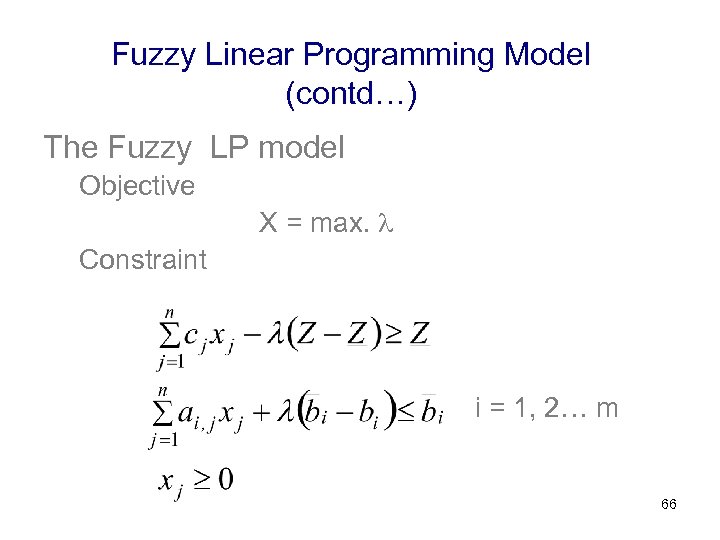Fuzzy Linear Programming Model (contd…) The Fuzzy LP model Objective X = max. Constraint i = 1, 2… m 66

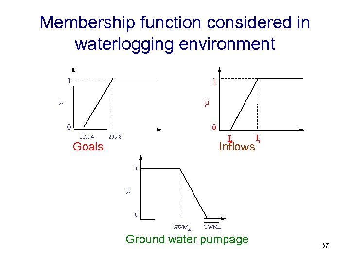Membership function considered in waterlogging environment 1 1 0 0 113. 4 Goals It 205. 8 Inflows It 1 0 GWMzt Ground water pumpage 67

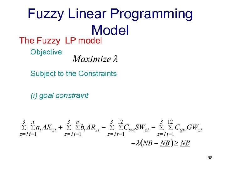Fuzzy Linear Programming Model The Fuzzy LP model Objective Subject to the Constraints (i) goal constraint 68

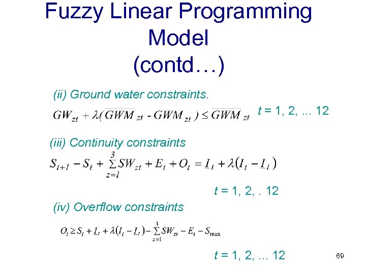Fuzzy Linear Programming Model (contd…) (ii) Ground water constraints. t = 1, 2, . . . 12 (iii) Continuity constraints t = 1, 2, . 12 (iv) Overflow constraints t = 1, 2, . . . 12 69

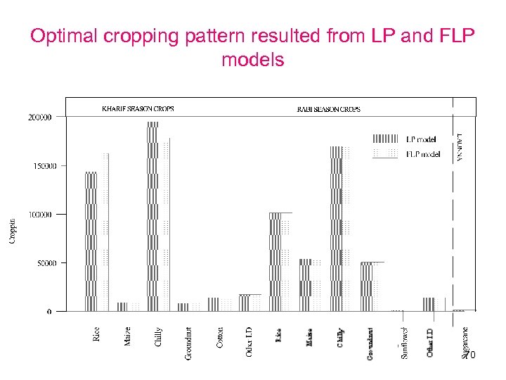Optimal cropping pattern resulted from LP and FLP models 70

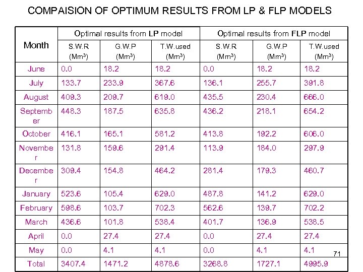COMPAISION OF OPTIMUM RESULTS FROM LP & FLP MODELS Optimal results from LP model Month S. W. R (Mm 3) G. W. P (Mm 3) Optimal results from FLP model T. W. used (Mm 3) S. W. R (Mm 3) G. W. P (Mm 3) T. W. used (Mm 3) June 0. 0 18. 2 July 133. 7 233. 9 367. 6 136. 1 255. 7 391. 8 August 409. 3 209. 7 619. 0 435. 5 230. 4 666. 0 Septemb er 448. 3 187. 5 635. 8 436. 2 218. 1 654. 2 October 416. 1 165. 1 581. 2 413. 8 192. 2 606. 0 Novembe 131. 8 r 159. 6 291. 4 113. 9 184. 0 297. 9 Decembe 309. 4 r 154. 8 464. 2 281. 4 179. 3 460. 7 January 523. 6 105. 4 629. 0 487. 8 141. 2 629. 0 February 598. 6 103. 7 702. 3 562. 6 139. 7 702. 2 March 436. 6 101. 8 538. 4 401. 7 136. 9 538. 5 April 0. 0 27. 4 May 0. 0 4. 1 Total 3407. 4 1471. 2 4878. 6 3268. 8 1727. 1 4995. 9 71

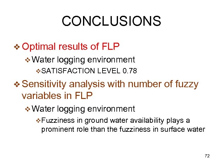CONCLUSIONS v Optimal v Water results of FLP logging environment v. SATISFACTION LEVEL 0. 78 v Sensitivity analysis with number of fuzzy variables in FLP v Water logging environment v. Fuzziness in ground water availability plays a prominent role than the fuzziness in surface water 72

Application case study – 4 Optimal operational plans for reservoir operation using GA 73

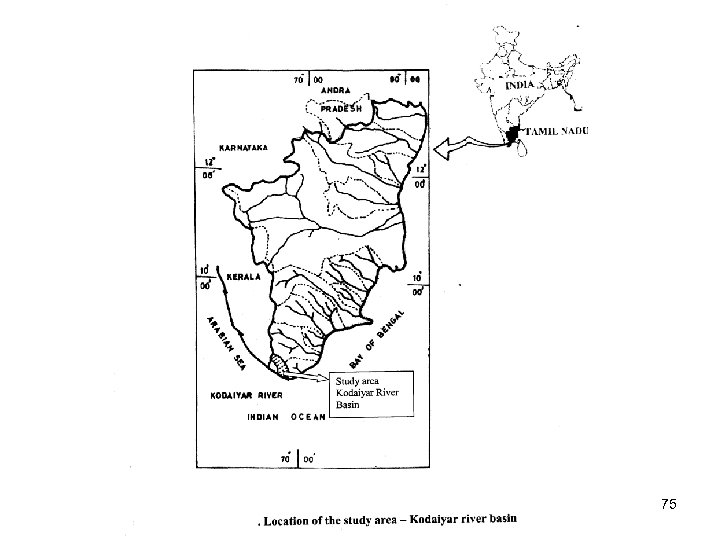
Single reservoir operating rule curves using GA • Pechiparai Reservoir System in the Kodaiyar river basin • The storage capacity of the Pechiparai Reservoir is 150 Mm³ with dead storage of 27 Mm 3 • 32 years of historical inflow data is used 74

75

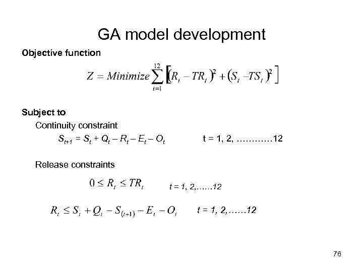GA model development Objective function Subject to Continuity constraint St+1 = St + Qt – Rt – Et – Ot t = 1, 2, ………… 12 Release constraints t = 1, 2, …… 12 76

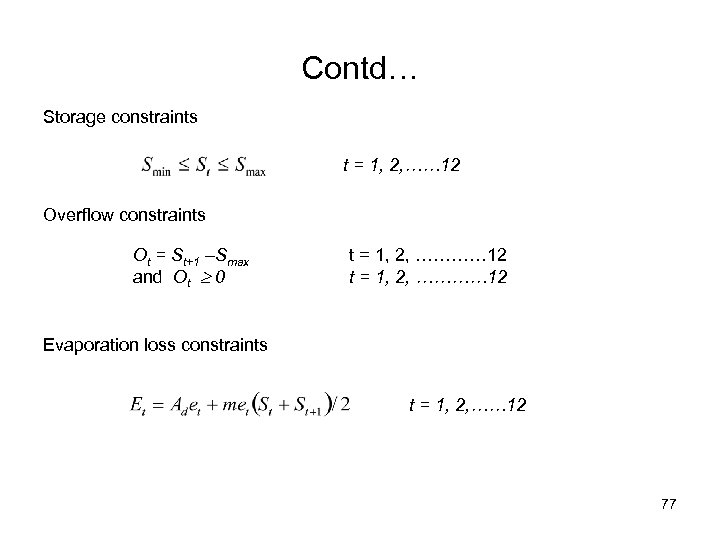Contd… Storage constraints t = 1, 2, …… 12 Overflow constraints Ot = St+1 –Smax and Ot 0 t = 1, 2, ………… 12 Evaporation loss constraints t = 1, 2, …… 12 77

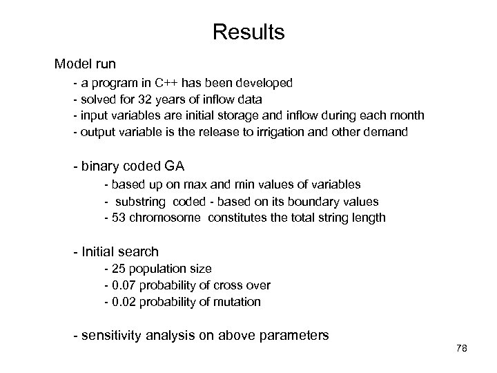Results Model run - a program in C++ has been developed - solved for 32 years of inflow data - input variables are initial storage and inflow during each month - output variable is the release to irrigation and other demand - binary coded GA - based up on max and min values of variables - substring coded - based on its boundary values - 53 chromosome constitutes the total string length - Initial search - 25 population size - 0. 07 probability of cross over - 0. 02 probability of mutation - sensitivity analysis on above parameters 78

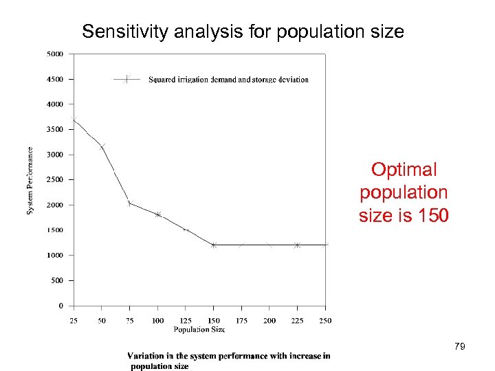Sensitivity analysis for population size Optimal population size is 150 79

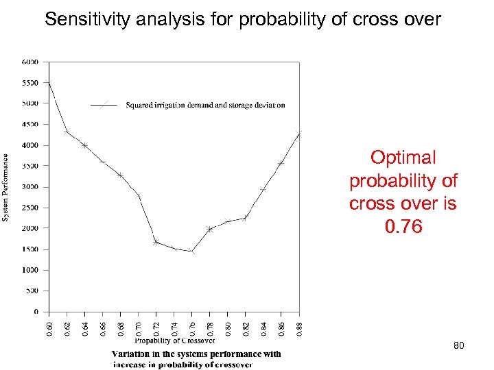Sensitivity analysis for probability of cross over Optimal probability of cross over is 0. 76 80

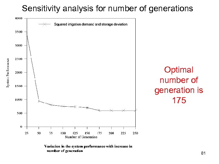Sensitivity analysis for number of generations Optimal number of generation is 175 81

Thus for the case study considered herein the optimal population is 150, optimal probability of cross over is 0. 76 and optimal number of generation is 175 82

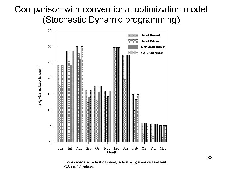Comparison with conventional optimization model (Stochastic Dynamic programming) 83

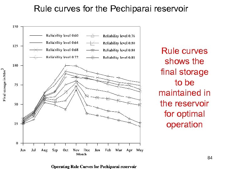Rule curves for the Pechiparai reservoir Rule curves shows the final storage to be maintained in the reservoir for optimal operation 84

Thank you 85