Vertical Weighting Functions Validation of Satellite Retrievals

Vertical Weighting Functions & Validation of Satellite Retrievals Chris Barnet NOAA/NESDIS/STAR (the office formally known as ORA) University of Maryland, Baltimore County (Adjunct Professor) AIRS Science Team Member NPOESS Sounder Operational Algorithm Team Member GOES-R Algorithm Working Group – Chair of Sounder Team NOAA/NESDIS representative to IGCO July 27, 2006 MSRI-NCAR Summer Workshop on Data Assimilation for the Carbon Cycle

Outline for Todays’s Lecture • A question from yesterday. – What are they. – How are they used. • Validation Techniques. – Discussion of observation types (mostly references). – Comparisons of CH 4 and CO 2 product with in-situ. • Summary of some papers on using AIRS CO 2 products in carbon assimilation systems. • Trace gas product correlations – A better way to use AIRS data? 2

A Question From Jeremy 1. What does the K matrix look like for temperature and moisture? 2. Why is there more vertical information about temperature than CO 2? 3

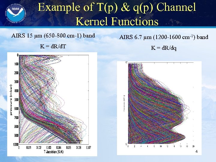Example of T(p) & q(p) Channel Kernel Functions AIRS 15 µm (650 -800 cm-1) band AIRS 6. 7 µm (1200 -1600 cm-1) band K = d. R/d. T K = d. R/dq 4

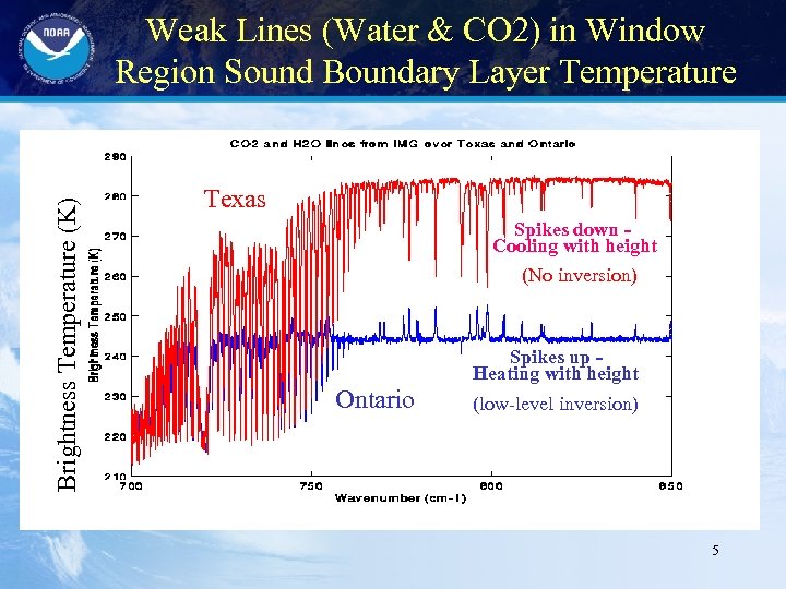Brightness Temperature (K) Weak Lines (Water & CO 2) in Window Region Sound Boundary Layer Temperature Texas Spikes down Cooling with height (No inversion) Spikes up Heating with height Ontario (low-level inversion) 5

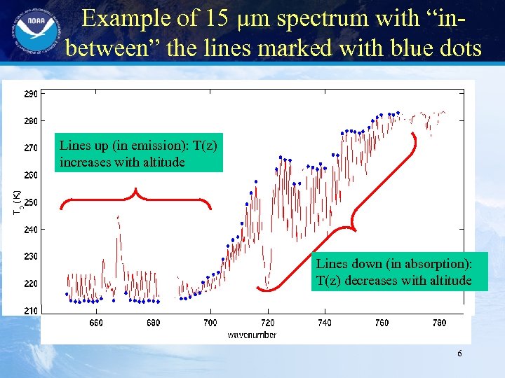Example of 15 µm spectrum with “inbetween” the lines marked with blue dots Lines up (in emission): T(z) increases with altitude Lines down (in absorption): T(z) decreases with altitude 6

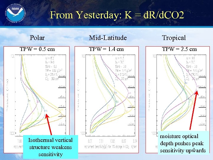From Yesterday: K = d. R/d. CO 2 Polar Mid-Latitude Tropical TPW = 0. 5 cm TPW = 1. 4 cm TPW = 2. 5 cm Isothermal vertical structure weakens sensitivity moisture optical depth pushes peak 7 sensitivity upwards

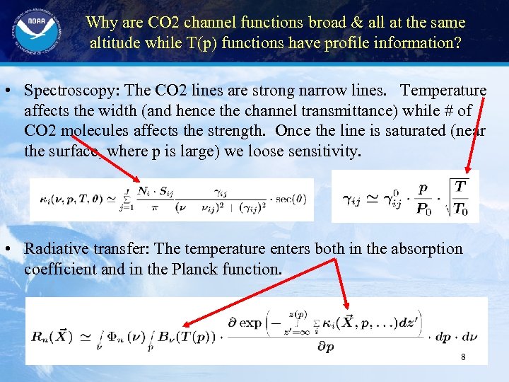Why are CO 2 channel functions broad & all at the same altitude while T(p) functions have profile information? • Spectroscopy: The CO 2 lines are strong narrow lines. Temperature affects the width (and hence the channel transmittance) while # of CO 2 molecules affects the strength. Once the line is saturated (near the surface, where p is large) we loose sensitivity. • Radiative transfer: The temperature enters both in the absorption coefficient and in the Planck function. 8

Why is CH 4 considered to be 25 x more powerful as a greenhouse gas than CO 2? 9

Why is CH 4 considered to be 25 x more powerful as a greenhouse gas than CO 2? • At 380 ppm the CO 2 lines are saturated and as CO 2 increases the absorption of energy changes as the log(N). • CH 4 is 1. 8 ppm and the lines are not saturated. As the amount of CH 4 changes the absorption is linear w. r. t # of molecules. 10

Retrieval Averaging Functions See 1) Rogers 2000, pg. 43 -44 & pg. 83 -85 2) Rodgers and Conner 2003 3) My notes – section 8. 12. 1 11

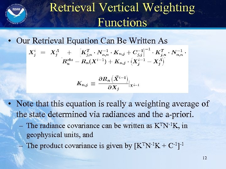Retrieval Vertical Weighting Functions • Our Retrieval Equation Can Be Written As • Note that this equation is really a weighting average of the state determined via radiances and the a-priori. – The radiance covariance can be written as KTN-1 K, in geophysical units, and – The product covariance is given by [KTN-1 K + C-1]-1 12

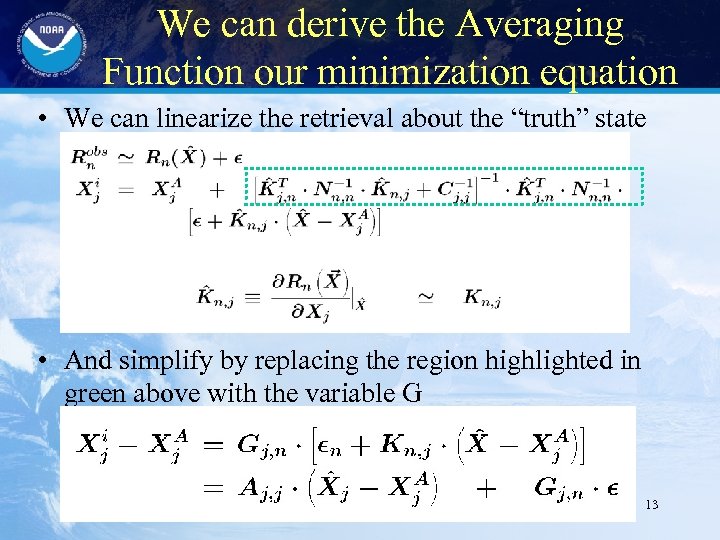We can derive the Averaging Function our minimization equation • We can linearize the retrieval about the “truth” state • And simplify by replacing the region highlighted in green above with the variable G 13

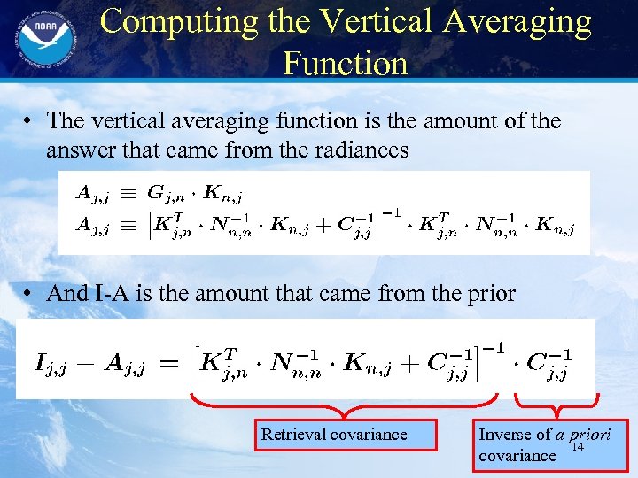Computing the Vertical Averaging Function • The vertical averaging function is the amount of the answer that came from the radiances • And I-A is the amount that came from the prior Retrieval covariance Inverse of a-priori 14 covariance

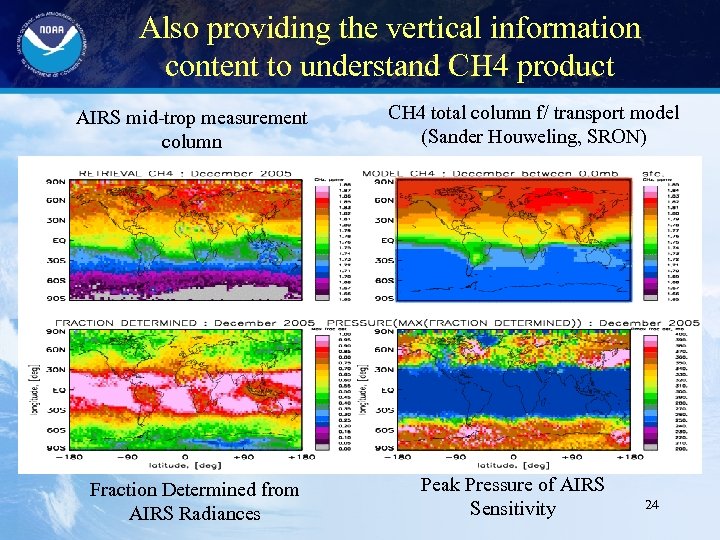
Value of the Vertical Averaging Function • A is the retrieval weighing of the channel kernel functions (think of a retrieval as an integrator of data) • A tells you how much the observations were believed. • I-A tells you how much of the a-priori was believed. • When comparing other measurements (such as high vertical resolution sondes or aircraft) the validation measurements – Must have similar vertical smoothing – Should be “degraded” by the fraction of the prior that entered the solution (i. e. , we know we can’t measure 100%) • When using AIRS products the A maxtrix – Tells you the vertical correlation between parameters – Tells you how much to believe the product and where to believe the product. – You can remove our a-priori assumptions and substitute your own. 15

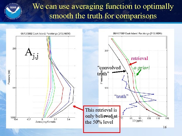We can use averaging function to optimally smooth the truth for comparisons Aj, j retrieval “convolved truth” a-priori “truth” This retrieval is only believed at the 50% level 16

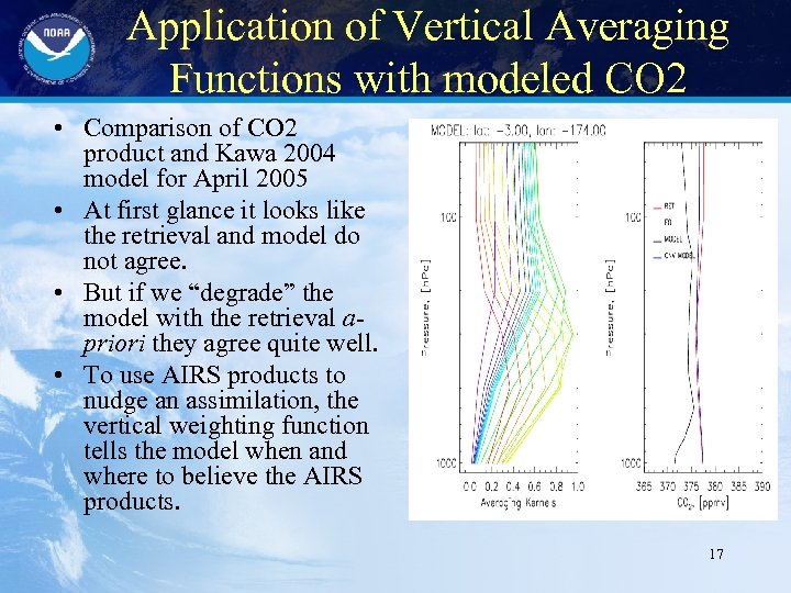Application of Vertical Averaging Functions with modeled CO 2 • Comparison of CO 2 product and Kawa 2004 model for April 2005 • At first glance it looks like the retrieval and model do not agree. • But if we “degrade” the model with the retrieval apriori they agree quite well. • To use AIRS products to nudge an assimilation, the vertical weighting function tells the model when and where to believe the AIRS products. 17

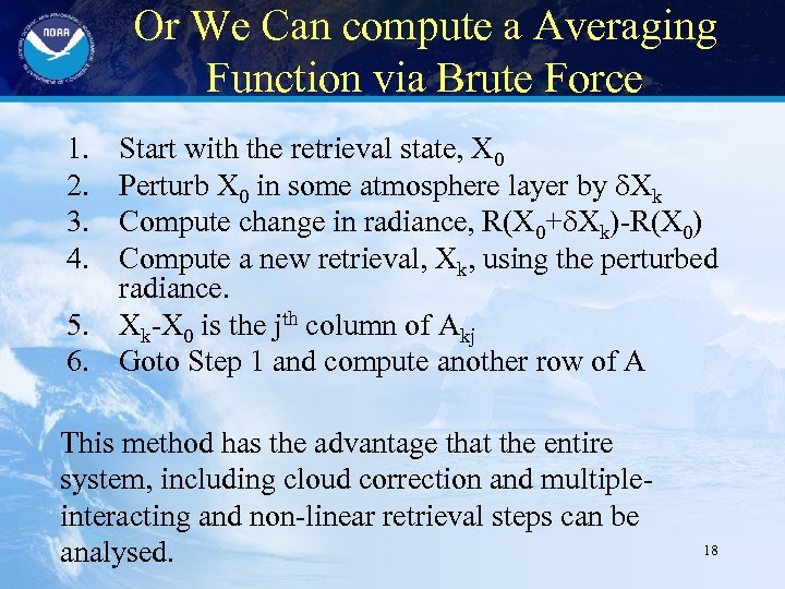Or We Can compute a Averaging Function via Brute Force 1. 2. 3. 4. Start with the retrieval state, X 0 Perturb X 0 in some atmosphere layer by Xk Compute change in radiance, R(X 0+ Xk)-R(X 0) Compute a new retrieval, Xk, using the perturbed radiance. 5. Xk-X 0 is the jth column of Akj 6. Goto Step 1 and compute another row of A This method has the advantage that the entire system, including cloud correction and multipleinteracting and non-linear retrieval steps can be analysed. 18

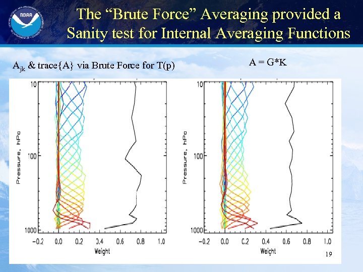The “Brute Force” Averaging provided a Sanity test for Internal Averaging Functions Ajk & trace{A} via Brute Force for T(p) A = G*K 19

Validation 20

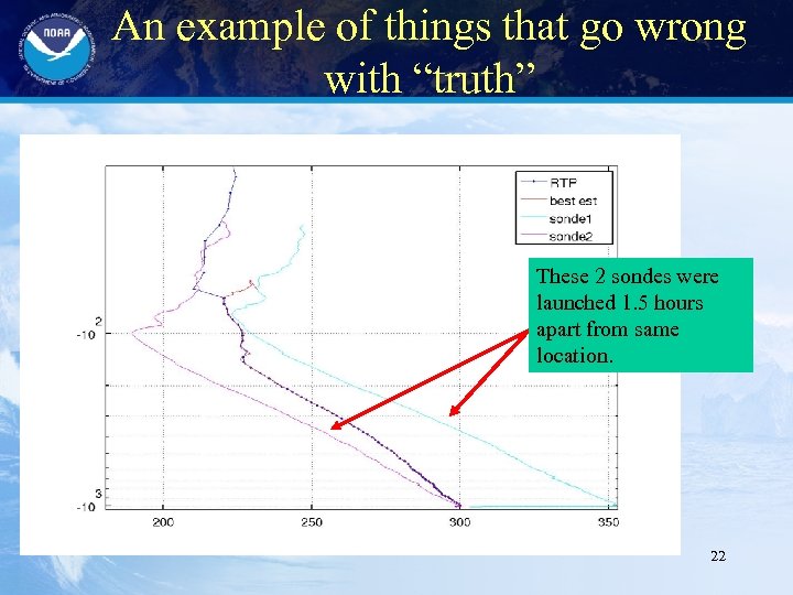
“what is truth” • Compare to ECMWF & NCEP Models (e. g. , See Susskind, 2005) – Can compare complete global dataset – Differences can be model or retrieval errors – Implicitly validating against all other instruments (space-borne, sondes, buoy’s etc. ) used in analysis • Compare to Radiosondes, Ozonesondes (e. g. , See Tobin, 2006, Divakarla, 2006) – Only a couple hundred “dedicated” sondes are flown per year. Usually we fly 2 sondes so we can see lower and upper air at overpass time. • Sondes can take 1 -2 hours to ascend • Sondes can drift up to 100’s of km’s – A few hundred sondes are launched globally per day that are within 300 km and +/- 1 hour of our overpass. • Different sonde instruments, quality of launches, etc. • In-situ intensive experiments with sondes, aircraft and LIDAR. – Have participated in INTEX-NA 6 AEROSE, START, MILAGRO, INTEX-B, AMMA 21

An example of things that go wrong with “truth” These 2 sondes were launched 1. 5 hours apart from same location. 22

Example of Validation of Methane Products from AIRS with ERSL/GMD surface flasks and aircraft 23

Also providing the vertical information content to understand CH 4 product AIRS mid-trop measurement column Fraction Determined from AIRS Radiances CH 4 total column f/ transport model (Sander Houweling, SRON) Peak Pressure of AIRS Sensitivity 24

Comparison of CH 4 product & ESRL/GMD Continuous Ground Site Barrow Alaska 3 deg. x 3 deg. gridded retrieval averaged over 60 -70 lat, & -165 to -90 lng 25

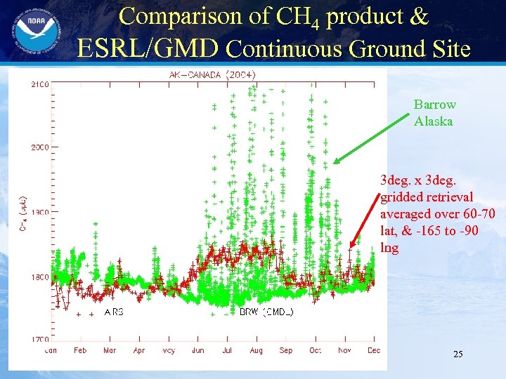
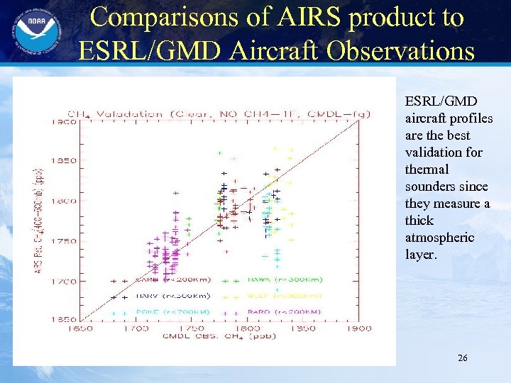Comparisons of AIRS product to ESRL/GMD Aircraft Observations ESRL/GMD aircraft profiles are the best validation for thermal sounders since they measure a thick atmospheric layer. 26

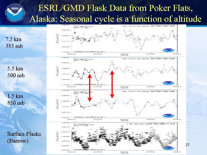ESRL/GMD Flask Data from Poker Flats, Alaska: Seasonal cycle is a function of altitude 7. 5 km 385 mb 5. 5 km 500 mb 1. 5 km 850 mb Surface Flasks (Barrow) 27

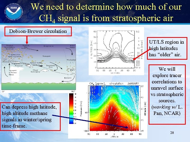We need to determine how much of our CH 4 signal is from stratospheric air Dobson-Brewer circulation UT/LS region in high latitudes has “older” air. Can depress high latitude, high altitude methane signals in winter/spring time-frame. We will explore tracer correlations to unravel surface vs stratospheric sources. (working w/ L. Pan, NCAR) 28

Example of Validation of Carbon Dioxide Products from AIRS with ESRL/GMD Marine Boundary Layer and Aircraft Products and Japanese Commercial Aircraft 29

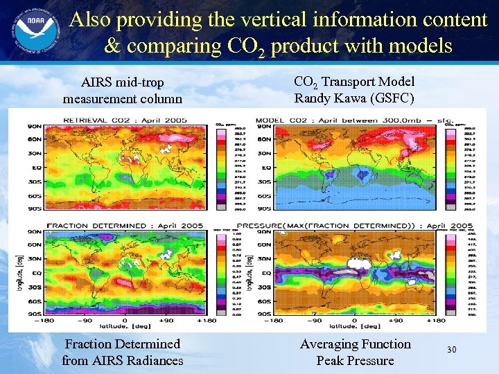Also providing the vertical information content & comparing CO 2 product with models AIRS mid-trop measurement column CO 2 Transport Model Randy Kawa (GSFC) Fraction Determined from AIRS Radiances Averaging Function Peak Pressure 30

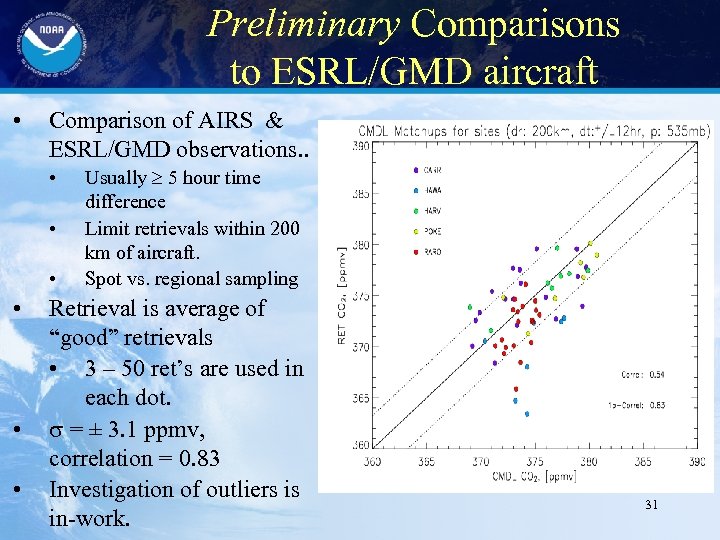Preliminary Comparisons to ESRL/GMD aircraft • Comparison of AIRS & ESRL/GMD observations. . • • • Usually 5 hour time difference Limit retrievals within 200 km of aircraft. Spot vs. regional sampling Retrieval is average of “good” retrievals • 3 – 50 ret’s are used in each dot. = ± 3. 1 ppmv, correlation = 0. 83 Investigation of outliers is in-work. 31

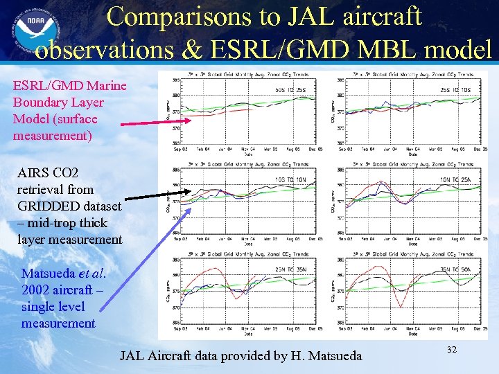Comparisons to JAL aircraft observations & ESRL/GMD MBL model ESRL/GMD Marine Boundary Layer Model (surface measurement) AIRS CO 2 retrieval from GRIDDED dataset – mid-trop thick layer measurement Matsueda et al. 2002 aircraft – single level measurement JAL Aircraft data provided by H. Matsueda 32

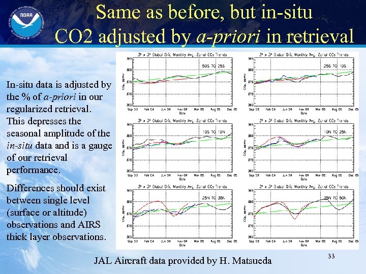Same as before, but in-situ CO 2 adjusted by a-priori in retrieval In-situ data is adjusted by the % of a-priori in our regularized retrieval. This depresses the seasonal amplitude of the in-situ data and is a gauge of our retrieval performance. Differences should exist between single level (surface or altitude) observations and AIRS thick layer observations. JAL Aircraft data provided by H. Matsueda 33

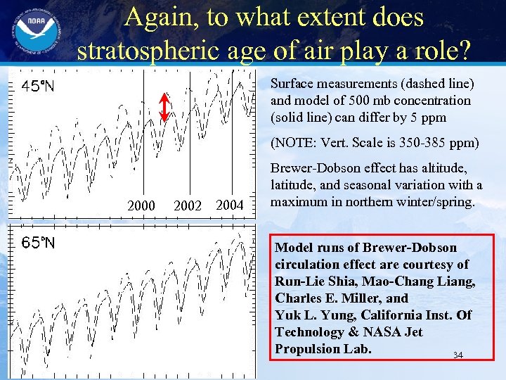Again, to what extent does stratospheric age of air play a role? Surface measurements (dashed line) and model of 500 mb concentration (solid line) can differ by 5 ppm (NOTE: Vert. Scale is 350 -385 ppm) 2000 2002 2004 Brewer-Dobson effect has altitude, latitude, and seasonal variation with a maximum in northern winter/spring. Model runs of Brewer-Dobson circulation effect are courtesy of Run-Lie Shia, Mao-Chang Liang, Charles E. Miller, and Yuk L. Yung, California Inst. Of Technology & NASA Jet Propulsion Lab. 34

Example of Validation of CO 2 measurements with Models 35

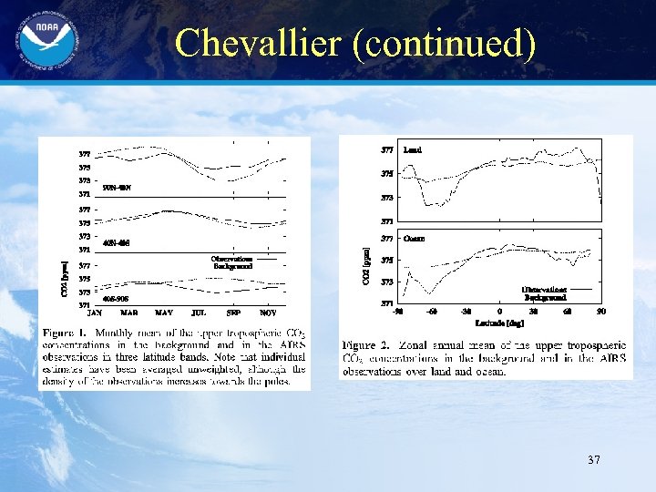
Chevallier, Engelen & Peylin, GRL, 2005 • Compared CO 2 derived from ECMWF 4 DVAR analysis of 18 AIRS channels (R. Engelen’s CO 2 product) vs Laboratoire de Météorologie Dynamique (LMDZ) GCM driven by surface flux climatology – Large systematic differences at high latitudes – Significant sea/land contrast – Use of a constant averaging kernel may contribute to biases. 36

Chevallier (continued) 37

Tiwari, et al. , JGR 2006 (in press) • CO 2 flux estimates of Rodenbeck 2003 used as boundary conditions for TM 3 (4 x 5 deg, 19 , NCEP winds) & LMDZ (2. 5 x 3. 75 deg, 19 , ECMWF winds) – Averaged monthly fluxes for 1993 -2001 and used as driver of transport for 2000 -2003 – Spun up model from Jan. 2000 -Dec. 2002 • Compared to R. Engelen’s product to explore two potential pathways for transport of CO 2 – North hemisphere mid-lat air laden w/ fossil fuel via northern high latitudes along upward sloping constant pot. Temp surfaces. – Dispersal of CO 2 laden air in the PBL toward the tropics and subsequent upwards via deep convection. • Conclusions – Models agree with each other more than with retrievals. – Hovmoeller diagrams (time vs latitude) show that models transport the CO 2 via the northern pathways whereas in the retrievals the CO 2 shows up instantaneously. 38 – More work is needed.

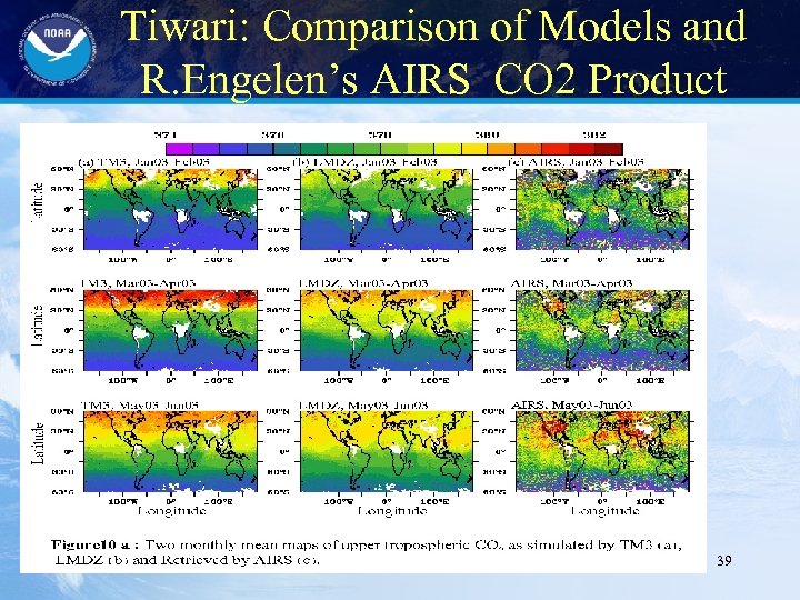Tiwari: Comparison of Models and R. Engelen’s AIRS CO 2 Product 39

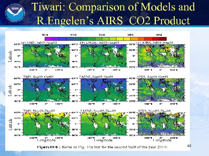Tiwari: Comparison of Models and R. Engelen’s AIRS CO 2 Product 40

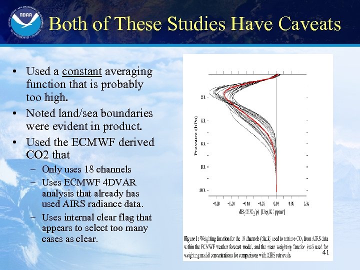Both of These Studies Have Caveats • Used a constant averaging function that is probably too high. • Noted land/sea boundaries were evident in product. • Used the ECMWF derived CO 2 that – Only uses 18 channels – Uses ECMWF 4 DVAR analysis that already has used AIRS radiance data. – Uses internal clear flag that appears to select too many cases as clear. 41

Can we “Validate” our Product Using Atmospheric Correlations Or Can AIRS product correlations have scientific value 42

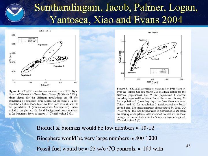Suntharalingam, Jacob, Palmer, Logan, Yantosca, Xiao and Evans 2004 Biofuel & biomass would be low numbers 10 -12 Biosphere would be very large numbers 800 -1000 Fossil fuel would be 25 w/o CO controls, 100 with 43

Pan, Wei, Kinnison, Garcia, Wuebbles, and Brasseur (submitted to JGR) • Using aircraft measurements of O 3, CO, and H 2 O in the upper troposphere/lower stratosphere to validate MOZART-3 & WACCM 3 model. – Chemical discontinuity at tropopause caused by changes in thermal and dynamic fields (Brewer. Dobson circulation) 44

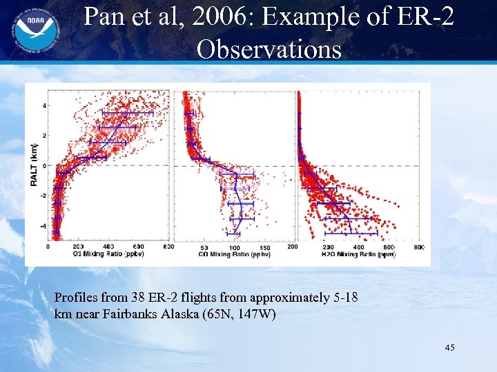Pan et al, 2006: Example of ER-2 Observations Profiles from 38 ER-2 flights from approximately 5 -18 km near Fairbanks Alaska (65 N, 147 W) 45

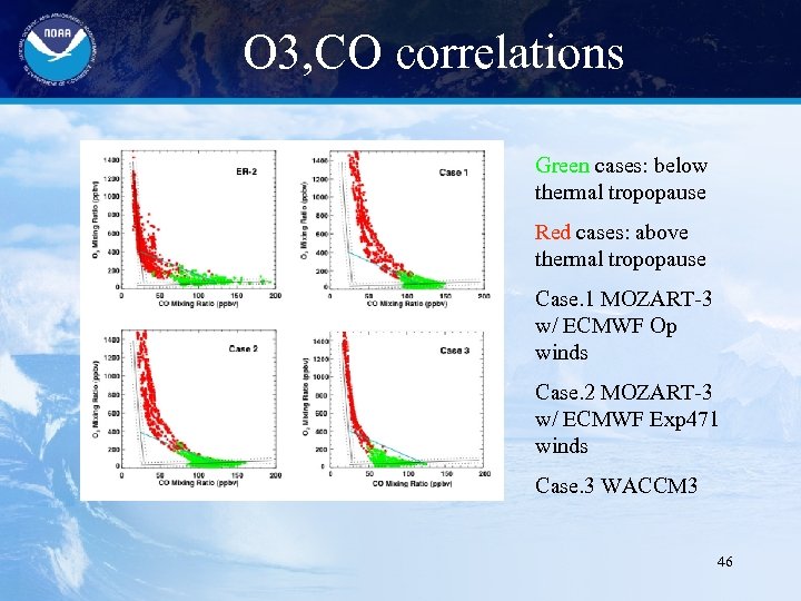O 3, CO correlations Green cases: below thermal tropopause Red cases: above thermal tropopause Case. 1 MOZART-3 w/ ECMWF Op winds Case. 2 MOZART-3 w/ ECMWF Exp 471 winds Case. 3 WACCM 3 46

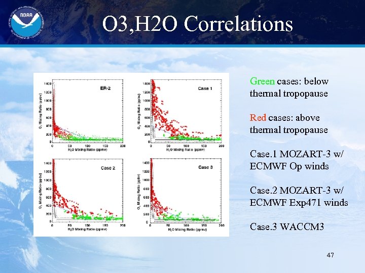O 3, H 2 O Correlations Green cases: below thermal tropopause Red cases: above thermal tropopause Case. 1 MOZART-3 w/ ECMWF Op winds Case. 2 MOZART-3 w/ ECMWF Exp 471 winds Case. 3 WACCM 3 47

So How Does This Relate to AIRS measurements? • We are collaborating with Laura Pan (NCAR) to compare AIRS products with Aircraft Products • We are computing correlations of AIRS products to see if we can distinguish air mass types. – Can we identify cases affected by Brewer-Dobson circulation and improve our ESRL/GMD & Matsueda comparisons? – Can we identify biomass regions and chemical conversion of CO? 48

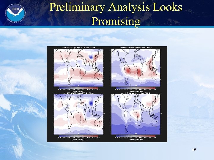Preliminary Analysis Looks Promising 49

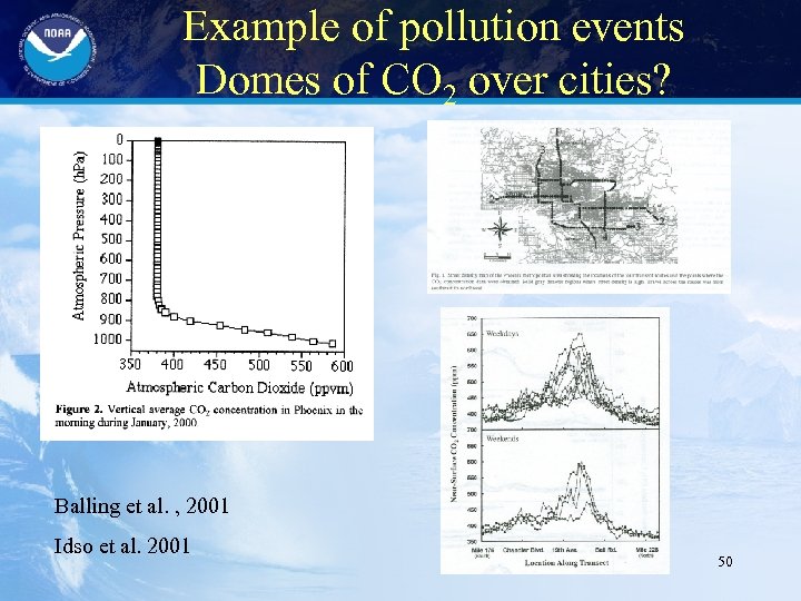Example of pollution events Domes of CO 2 over cities? Balling et al. , 2001 Idso et al. 2001 50

So maybe the utility of thermal sounders has yet to be exploited • AIRS has measured global tropospheric CO 2 & CH 4 for the first time. • AIRS has a unique capability to intercompare tropospheric products of temperature, water, O 3, CO, CH 4, and CO 2. • We expect to learn new things from this dataset. • We are exploring diurnal signals and hope to identify large pollution or biosphere events over the lifetime of these instruments. • We are exploring the use of trace gas correlations within the AIRS products. • We want to work with transport modelers to compare our product to a realistic emission scenario for CO 2 with proper vertical weighing functions. • Other ideas? 51

References AIRS Instrument & Retrieval Algorithms • Aumann, H. H. , M. T. Chahine, C. Gautier, M. D. Goldberg, E. Kalnay, L. M. Mc. Millin, H. Revercomb, P. W. Rosenkranz, W. L. Smith, D. H. Staelin, L. L. Strow and J. Susskind 2003. AIRS/AMSU/HSB on the Aqua mission: design, science objectives, data products, and processing systems. IEEE Trans. Geosci. Remote Sens. v. 41 p. 253 - 264. {PDF FILE = Aumann_IEEE 8 big 15 aug 02. pdf} • Susskind, J. , C. D. Barnet, J. M. Blaisdell, L. Iredell, F. Keita, L. Kouvaris, G. Molnar and M. T. Chahine 2006. Accuracy of geophysical parameters derived from Atmospheric Infrared Sounder Advanced Microwave Sounding Unit as a function of fractional cloud cover. J. Geophys. Res. v. 111 doi: 10. 1029/2005 JD 006272, 19 pgs. {PDF FILE = 2005 JD 006272_susskind. pdf} • Susskind, J. , C. D. Barnet and J. M. Blaisdell 2003. Retrieval of atmospheric and surface parameters from AIRS/AMSU/HSB data in the presence of clouds. IEEE Trans. Geosci. Remote Sens. v. 41 p. 390 -409. {PDF FILE = susskind_IEEE 23 apr 02 sub. pdf} • Rodgers, C. D. 2000. Inverse methods for atmospheric sounding: Theory and practice. World Scientific Publishing 238 pgs. 52

References Analysis of AIRS C products • Barkley, M. P. , P. S. Monks and R. J. Engelen 2006. Comparison of SCIAMACHY and AIRS CO 2 measurements over North America during the summer and autumn of 2003. Geophys. Res. Lett. (in press). {PDF FILE = grl_fsi_v 1. pdf} • Chevallier, F. , R. J. Engelen and P. Peylin 2005. The contribution of AIRS data in the estimation of CO 2 sources and sinks. Geophys. Res. Lett. v. 32 L 23801 doi: 10. 1029/2005 GL 024229, 4 pgs. {PDF FILE = 05 chevallier_publ. pdf} • Tiwari, Y. K. , M. Gloor, R. J. Engelen, F. Chevallier, C. Rodenbeck, S. Korner, P. Peylin, B. H. Braswll and M. Heimann 2006. Comparing CO 2 retrieved from AIRS with model predictions: implications for constraining surface fluxes and lower to upper tropospheric transport. J. Geophys. Res. (in press). – Rodenbeck, C. , S. Houweling, M. Gloor and M. Heimann 2003. CO 2 flux history 1982 -2001 inferred from atmospheric data using a global inversion of atmospheric transport. Atmos. Chem. Phys. v. 3 p. 1919 -1964. {PDF FILE = acp-3 -1919. pdf} 53

References AIRS Trace Gas Algorithms • Haskins, R. D. and L. D. Kaplan 1993. Remote sensing of trace gases using the atmospheric infrared sounder. Intl Rad. Symp. (QC 912. 3 I 57 1992, Deepak Publ. ) p. 278 -281. {PDF FILE = haskins_kaplan_1992. pdf} • Crevoisier, C. , S. Heilliette, A. Chedin, S. Serrar, R. Armante and N. A. Scott 2004. Midtropospheric CO 2 concentration retrieval from AIRS observations in the tropics. Geophys. Res. Lett. v. 31 p. 1710617110. doi: 10. 1029/2004 GL 020141 {PDF FILE = 2004 GL 020141. pdf} • Crevoisier, C. , A. Chedin and N. A. Scott 2003. AIRS channels selection for CO 2 and other trace gases retrieval. Quart. J. Roy. Meteor. Soc. v. 128 p. 2719 -2740. doi: 10. 1256/qj. 02. 180 {PDF FILE = 03 qjrms_airs_chl. pdf} • Engelen, R. J. and A. P. Mc. Nally 2005. Estimating atmospheric CO 2 from advanced IR satellite radiances within an operational 4 D-Var data assim. system: Results and Validation. J. Geophys. Res. v. 110 D 18305 doi: 10. 1029/2005 JD 005982 {PDF FILE = 2005 JD 005982_engelen. pdf} • Engelen, R. J. and G. L. Stephens 2004. Information content of infrared satellite sounding measurements with respect to CO 2. J. Appl. Meteor. v. 43 p. 373 -378. {PDF FILE = Engelen_jap 2004. pdf} • Engelen, R. J. , G. L. Stephens and A. S. Denning 2001. The effect of CO 2 variability on the retrieval of atmospheric temperatures. Geophys. Res. Lett. v. 28 p. 3259 -3263. {PDF FILE =2001 GL 013496_engelen. pdf} 54

References Averaging Functions & Validation • Divakarla, M. G. , C. D. Barnet, M. D. Goldberg, L. M. Mc. Millin, E. Maddy, W. W. Wolf, L. Zhou and X. Liu 2006. Validation of Atmospheric Infrared Sounder temperature and water vapor retrievals with matched radiosonde measurements and forecasts. J. Geophys. Res. v. 111 D 09 S 15 doi: 10. 1029/2005 JD 006116, 20 pgs. {PDF FILE = 2005 JD 006116. pdf} • Gettelman, A. , E. M. Weinstock, E. J. Fetzer, F. W. Irion, A. Eldering, E. C. Richard, K. H. Rosenlof, T. L. Thompson, J. V. Pittman, C. R. Webster and R. L. Herman 2004. Validation of Aqua satellite data in the upper troposphere and lower stratosphere with in situ aircraft. Geophys. Res. Lett. v. 31 L 22107 doi: 10. 1029/2004 GL 020730 {PDF FILE = Gettelman 2004 GL 020730. pdf} • Houweling, S. , F. Dentener, J. Lelieveld, B. P. Walter and E. J. Dlugokencky 2000. The modeling of tropospheric methane: How well can point measurements be reproduced by a global model. J. Geophys. Res. v. 105 p. 8981 -9002. {PDF FILE = 1999 JD 901149. pdf} • Houweling, S. 2000. Global modeling of atmospheric methane sources and sinks. Ph. D Dissertation 177 pgs. {PDF FILE = houweling_thesis. pdf} • Kawa, S. R, D. J. Erickson III, S. Pawson and Z. Shu 2004. Global CO 2 transport simulations using meteorological data from the NASA data assimilation system. J. Geophys. Res. v. 109 D 18312 doi: 10. 1029/2004 J 004 554, 17 pgs. {PDF FILE = 2004 JD 004554_kawa. pdf} • Rodgers, C. D. and B. J. Conner 2003. Inter-comparison of remote sounding instruments. J. Geophys. Res. v. 108 p. 1 -14. doi: 10. 1029/2002 JD 002299 {PDF FILE = 03 JGR_Rodgers. pdf} • Tobin, D. C. , H. E. Revercomb, C. C. Moeller and T. S. Pagano 2006. Use of Atmospheric Infrared Sounder high spectral resolution spectra to assess the calibration of Moderate resolution Imaging Spectroradiometer on EOS Aqua. J. Geophys. Res. v. 111 D 09 S 05 doi: 10. 1029/2005 JD 006095, 15 pgs. {PDF FILE = 2005 JD 006095. pdf} • Tobin, D. C. , H. E. Revercomb, R. O. Knuteson, B. L. Lesht, L. L. Strow, S. E. Hannon, W. F. Feltz, L. A. Moy, E. J. Fetzer and T. S. Cress 2006. Atmospheric Radiation Measurement site atmospheric state best estimates for Atmospheric Infrared Sounder temperature and water retrieval validation. J. Geophys. Res. v. 111 D 09 S 14 doi: 10. 1029/2005 JD 006103, 18 pgs. {PDF FILE = 2005 JD 006103. pdf} 55

References Circulation & Gas Correlations • Shia, R. L. , M. C. Liang, C. E. Miller and Y. L. Yung 2006. CO 2 in the upper troposphere: influence of stratosphere-troposphere exchange. Geophys. Res. Lett. v. 33 L 14814 doi: 10. 1029/2006 GL 026141, 4 pgs. {PDF FILE = 2006 GL 026141_shia. pdf} • Palmer, P. I. , P. Suntharalingam, D. B. A. Jones, D. J. Jacob, D. G. Streets, Q. Fu, S. A. Vay and G. W. Sachse 2006. Using CO 2: CO correlations to improve inverse analyses of carbon fluxes. J. Geophys. Res. v. 111 D 12318 doi: 10. 1029/2005 JD 006697, 11 pgs. {PDF FILE = 06 jgr_palmer_co_co 2. pdf} • Suntharalingam, P. , D. J. Jacob, P. I. Palmer, J. A. Logan, R. M. Yantosca, Y. Xiao and M. J. Evans 2004. Improved quantification of Chinese carbon fluxes using CO 2/CO correlations in Asian outflow. J. Geophys. Res. v. 109 D 18 S 18 doi: 10. 1029/2003 JD 004362, 13 pgs. {PDF FILE = 2003 JD 004362_suntha. pdf} 56

References CO 2 Domes, Fossil Fuel Use • Balling Jr. , R. C. , R. S. Cerveny and C. D. Idso 2001. Does the urban CO 2 dome of Phoenix, Arizona contribute to its heat island? Geophys. Res. Lett. v. 28 p. 4599 -4601. {PDF FILE = 2000 GL 012632. pdf} • Idso, C. D. , S. B. Idso and R. C. Balling Jr. 2001. Intensive two-week study of an urban CO 2 dome. Atmospheric Environment v. 35 p. 995 -1000. {PDF FILE = 01_idso_domes. pdf} • Deffeyes, Kenneth 2005. Beyond oil: The view from Hubbert's peak. Hill and Wang, (div of Farrar, Straus and Giroux) NYC 202 pgs. • Deffeyes, Kenneth 2001. Hubbert's peak: the impending world oil shortage. Princeton University Press 208 pgs. • Eshel, G. and P. A. Martin 2006. Diet, energy, and global warming. Earth Interactions v. 10 p. 1 -17. {PDF FILE = 06 ei_eshel. pdf} • Eshel, G. and P. A. Martin 2006. Diet, energy, and global warming. BAMS v. 5 p. 562 -562. {PDF FILE = 0605 bams_diet_energy. pdf} 57