Verification of Daily CFS forecasts Huug van den

Verification of Daily CFS forecasts Huug van den Dool & Suranjana Saha • CFS was designed as ‘seasonal’ prediction system • Hindcasts 1981 -2005, 15 ‘members’ per month • Here we look at CFS(T 62 L 64) as NWP (never mind the delayed ocean analysis) • 25 years of forecasts (4500 forecasts out to 9 months) by a ‘constant’ T 62 L 64 model !!!!!. website http: //cfs. ncep. noaa. gov/ • Reference: S. Saha, S. Nadiga, C. Thiaw, J. Wang, W. Wang, Q. Zhang, H. M. van den Dool, H. -L. Pan, S. Moorthi, D. Behringer, D. Stokes, M. Pena, S. Lord, G. White, W. Ebisuzaki, P. Peng, P. Xie , 2006 : The NCEP Climate Forecast System. Journal of Climate, Vol. 19, No. 15, pages 3483. 3517 • • Today: No ensemble averages, hardly time averages One could compare to similarly large data sets, such as: CDAS & CDC’s MRF & ECMWF ‘monthly’ system : Cathy Thiaw (reruns) Acknowledgement and on CDAS info Bob Kistler/Fanglin Yang/Pete Caplan

Issues • • • Day-5 scores Climatology of scores Bias Correction (mean, sd) NH/SH/TR; Z 500, PSI 200, CHI 200 wk 3, wk 4, MJO Lorenzian Error growth equation The perfect forecast Scores as function of a) space, b) EOF mode Steps to improve signal to noise ratio FUTURE (CFSRR)

NCEP’s NEW CFS Components for S/I Climate • T 62/64 -layer version of the ~2003 NCEP atmospheric GFS (Global Forecast System) model – – – – Model top 0. 2 mb Simplified Arakawa-Schubert convection (Pan) Non-local PBL (Pan & Hong) SW radiation (Chou, modifications by Y. Hou) Prognostic cloud water (Moorthi, Hou & Zhao) LW radiation (GFDL, AER in operational wx model) R 2 Initial conditions for Atmosphere&Land • GFDL Modular Ocean Model, version 3 (MOM-3) – 40 levels – 1 degree resolution, 1/3 degree on equator • Global Ocean Data Assimilation (GODAS) • Fully coupled atmosphere-ocean (no flux correction)

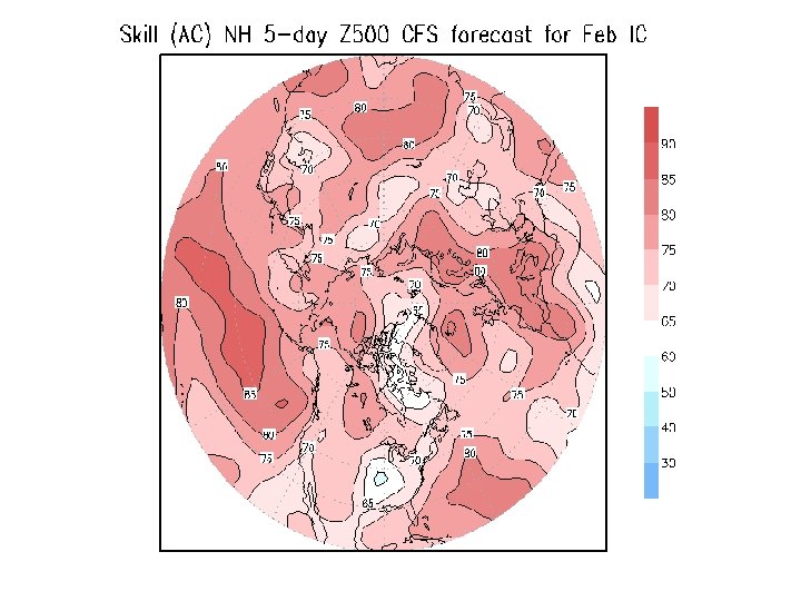
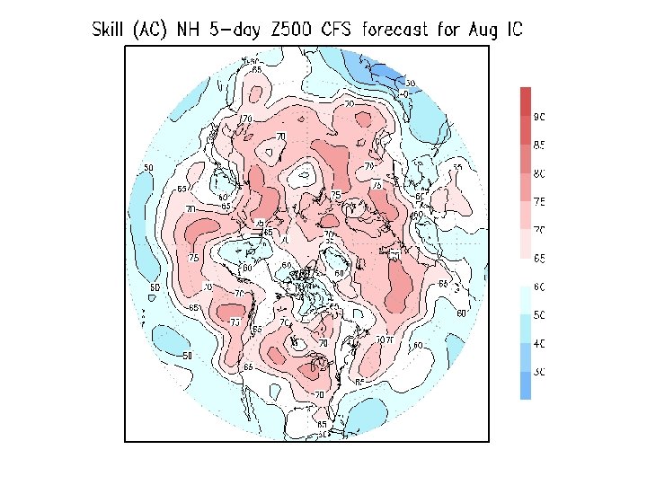
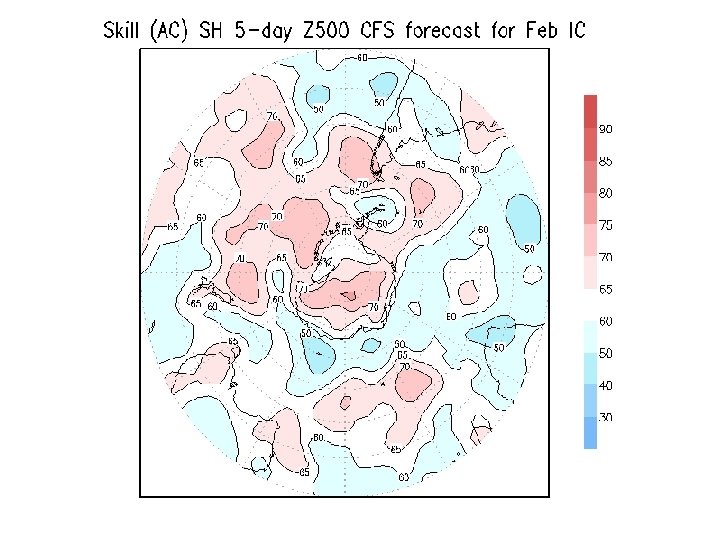
Day 5 AC-scores, using the harmonically smoothed model and observed climatologies (which are more ‘competitive’ than the old-old monthly climo used on Pete Caplan’s page Variables: Extra-tropical Z 500 (NH, SH) PSI 200 and CHI 200

Forecast Lead time [Hrs] 6480 168 144 120 96 72 48 24 o o o o 30 31 1 2 3 o o o o o o o o o o o o o o o o o o 9 10 11 12 13 o o o o o o o o o o o o o o o o o 19 20 21 22 23 o o o o o o o o o o o o Time [Days]

Fig. 2. The climatological annual cycle of the mean value of the geopotential height at a grid point close to Washington, DC, is shown as a smooth red curve. Shown are both the observed climatology (left panel) and the forecast climatology at a lead of 6480 hours (~ 9 months) (right panel). The 24 -yr mean values as calculated directly from the data are shown by the blue curves. The reason for the discontinuities in the right panel is that these values are only available during roughly half of the days in a year. The time on the abscissa in the right panel is the initial time of the forecast, not the actual time when the forecast is valid. In this case this implies an offset by roughly nine months. Unit is m. ACKNOWLEDGEMENT: Ake Johansson

Day 5 AC-scores, using the harmonically smoothed model and observed climatologies (which are more ‘competitive’ than the old-old monthly climo used on Pete Caplan’s page Variables: Extra-tropical Z 500 (NH, SH) PSI 200 and CHI 200

180 forecasts per dot Z 500: 72. 3 (4500 cases, grand mean) Congratulations with a constant system!

From Pete Caplan’s EMC website: 0. 7 Grand Mean NH over 1984 -2005: 70. 5 (CDAS 1) ((CDAS statistics has several problems)) 0. 7

CDAS

CFS

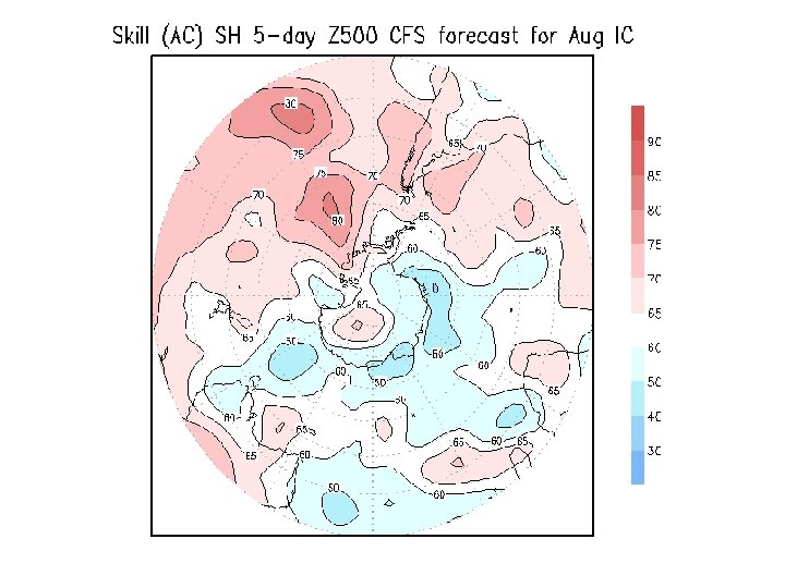
Next Two Slides: Excursion to SH Z 500

SH (CFS) Z 500: 62. 9 (4500 cases, grand mean) Scores ‘volatile’ in SH (still 180 per dot) Scores go UP and UP! “Congratulations” to whom ? ? ?

SH (CDAS)

Doing the best we can: Comparing CFS to CDAS day 5 Z 500 scores) NH CFS 1981 -2005 0. 723 T 62 L 64, coupled, R 2, harmonic daily climo CDAS 1984 -2005 0. 705 T 62 L 28, R 1, ‘old’ monthly climo SH 0. 629 0. 623 Flawed Warning: Number of forecasts per month differ. Climos differ!!! and change in ’ 96 for CDAS

Prelim Conclusion • R 2/CDAS 2/CFS 5 -day forecasts are (slightly) better than R 1/CDAS. • NH much better than SH (typical for pre 2000 technology) – this will change largely in next CFSRR (Jan 2010? ? ) • Trend-issues and non-constancy of system (will get worse)

Next Two Slides: Excursion to TROPICS

ENSO? 180 forecasts per dot PSI 200: 63. 0 (4500 cases grand mean) No increase? ? ?

ENSO? 180 forecasts per dot CHI 200: 45. 9 (4500 cases grand mean) This may be lowish for MJO type prediction. Definitely no increase over time. Perhaps a decrease!!!

Climatological Annual Cycle of day-5 scores

NH: Best month is Feb (76. 4), Worst month is July (67. 7). Near sinusoidal variation. Range=8. 7 pnts NH SH: Best month is Aug (64. 9), Worst month is March (59. 0). Typically 62 -64, except Feb-Apr. Range=5. 9 pnts Should we be surprised that the winter-summer difference in NH is NOT larger!? ? SH Forecasts verifying in month shown Curious: March is best/worst in NH/SH. Aug is best/worst in SH/NH. 375 forecasts per month

The NH has an annual cycle in skill, every year. (Each color curve is a different year. ) The SH does NOT have a clear annual variation in skill each year. 15 forecasts per month

forecasts verifying in month shown 375 forecast per dot(month) Large annual variation in the tropics! But volatile.

How about Bias Correction? ? ? One of the claimed usages of hindcasts

Based on 375 forecasts. Indisputable but very small improvement. Is Z 500 incorrigeable? The looks of a die-off curve

The gain due to bias correction in a few selected months. Day 5 scores Z 500 1981 -2005 Raw Bias Corrected NH DEC 73. 0 74. 5 (+1. 5) NH JUL 65. 8 68. 3 (+2. 5) SH FEB 61. 8 63. 5 (+1. 7) SH AUG 62. 2 63. 7 (+1. 5)

Is Z 500 incorrigeable? Largely Yes, because the systematic error is small. Wait till you see CHI 200

Chi 200 improves tremendously from cleaning up the bias, especially early on. 375 forecasts Can we do MJO forecasts ? ?

PSI 200 in Tropics does not improve very much from bias removal. !!!! The looks of a die-off curve

Day 5 scores • AC (obviously; already shown), But also: • SD • e. DOF

CFS misses 5 -20 % of variability Loss of variance does not increase beyond 10 -15 days and is never more than 20%

CFS misses several degrees of freedom Loss of does not increase beyond 10 -15 days and is never more than shown above

Compare the SD reduction in the NH To that in the SH

Compare the DOF reduction in the NH To that in the SH

The climatological AC variation can be explained by e. DOF and sd: low dof > high score, high sd > high score.

Distribution of Skill in space is important and largely unexplored and unexplained (because we never had enough data)

Skill as a function of (EOF) mode is interesting

Now: OUT TO 270 DAYS !!

Die-off curve, Z 500, NH, 1981 -2005, 4500 forecasts, all seasons aggregated Detail: Month 2 to Month 8 Detail, first month. NH

Die-off curve, Z 500, SH, 1981 -2005, 4500 forecasts, all seasons aggregated SH

FOCUS • • • Week 3 Week 4 = days 15 -21 and 22 -28 Physical basis of wk 3/wk 4 Ocean interaction is as much a liability as a promise at this point in time.

DAY 15 DAY 28 CFS Pers NH 15. 2 4. 2 6. 1 TR 36. 2 29. 3 29. 6 27. 5 SH 9. 6 2. 0 6. 2 3. 9 3. 4 Anomaly correlation of CFS and ‘Persistence’ Z 500 prediction in Feb 1981 -2005

signal ___________ ratio NOISE Improving signal to noise ratio: (often cosmetic) by reducing noise by applying some operator and, hopefully, not hurting the signal by this operator 1) Take a time mean (7 days) 2) Ensemble mean (not done here) 3) EOF filters (or better (maximally predictable modes))

Effect of a 7 day mean……… Day 15 Wk 3 Wk 4 Day 28 NH 15. 2 15. 7 9. 2 TR 36. 2 46. 7 42. 9 29. 6 SH 9. 6 10. 6 5. 2 6. 1 2. 0 Anomaly correlation of CFS Z 500 prediction, daily as well as weekly, in Feb 19812005

Effect of EOF truncation…… Wk 3 WK 4 EOF 1 -10 WK 4 EOF 1 -10 15. 7 22. 0 23. 9 18. 7 9. 2 12. 0 So, overall, we went from daily scores (15. 2…. 6. 1) to weekly scores (15. 7 and 9. 2) to filtered weekly scores (22. 0 and 23. 9 at best)

15. 7

9. 2

Longer time average, and N member ensemble average helps. From Wanqiu Wang’s page. Constructed Analogue

Initial error=6. 1 gpm ; Systematic error growth s=13. 5 gpm/day ; Small error amplification a=0. 181/day ; e-infinity=157. 7 gpm ; NOSEC

Savijarvi’s equation 5: Lorenz Tellus 1982

Initial error=4. 7 gpm ; Systematic error growth s=13. 1 gpm/day ; Small error amplification a=0. 181/day ; e-infinity=155. 7 gpm ; SEC

Initial error=4. 7 gpm ; Systematic error growth s=12. 6 gpm/day ; Small error amplification a=0. 200/day ; e-infinity=158. 3 gpm ; SECSD

Among 4500 CFS daily forecasts: • Was the RMSE at day 4 ever smaller than at day 3? ? ? (Model vs Analysis) • Yes, in one single case: the forecast from Dec, 31, 2003. Raise the champagne? ? ?

1 AC 2 3 4 5 6 9 98. 8 98. 6 97. 9 98. 5 97. 0 91. 6 RMSE 17. 1 20. 2 24. 6 20. 5 27. 4 45. 2 Jan 1 87. 9 Jan 5 An exceptionally “good” forecast, especially for T 62 (CDAS 2). The best forecast (for day 5) ever seen in this building, by any model Flow Situation is NOT particularly persistent Forecasts from Dec 30 or Jan 1, 2 are not that good. Only Dec 31, 0 Z. Other models not that good for this case Too good to be true? The date raises some suspicion

Due to Fanglin Yang

Another piece of evidence: • Scores in the SH for 2003123100 were also exceptionally good (0. 92, 2 nd highest is 0. 77). • It is unlikely that both hemispheres produce ‘hit-the-jackpot’ type forecasts. • Could something be the matter with the R 2 analyses.

What could be wrong in the (R 2 or any) analyses verifying the CFS forecast from 31 Dec, 0 Z? ? • Drunken observers around the planet in a wave-like pattern (New Years Eve distracts! • Satellites flying in and out of the year (in local time), i. e. time problems. Indeed much satellite data is rejected (for days in early January), sometimes ‘wholesale’. • But can this derail the analysis enough to explain a ‘very good’ forecast?

ABOUT THE FUTURE

5 day forecast anomaly correlation Annual Mean Reanalysis NH SH OPR 85 80 CFSRR-lite 74 72 CFS (R 2) 72 63 R 1 71 62

Conclusions • CFS is (slightly) better than CDAS (Z 500). • Over time (1981 -2005), the CFS “system” appears quite constant with various qualifiers • If we need an as-constant-as possible in-house system, look no further than CFS (better than CDAS) • Bias correction: small +ve impact on Z 500 and Ψ 200 (1 -2 pnts) • Bias correction: huge +ve impact on CHI-200 (15 pnts), but this is worrisome • CFS loses 5 -20% in terms of SD and e. DOF in the first few days, then, admirably, stays nearly constant out to 270 days

More conclusions • • Scores in SH/TR more volatile than in NH. SH lacks a proven annual cycle in scores Spatial distribution of scores not easy to understand Chi 200 scores at day 1 point to serious problems in R 2 and ‘consistency’ • Scores as a function of EOF non-surprising • Error growth equation fits (Lorenz/Savijarvi) indicates large (mainly random) error growth due to systematic model error. Surprising. Needs more study. The good news about it is …. . • We have one perfect forecast.

More Conclusions • (Very) modest skill in wk 3 and wk 4 • Even with 2 of 3 steps for signal to noise improvements in place, the AC is only 0. 20 -0. 25. (No ensemble average here) • Waiting for the next CFS and CFSRR (higher Res, consistent IC)

Conclusions: • The day 1 – 3 forecasts appear to be too damped, and damp faster than a regression would. Increasing anomaly amplitude as a postprocessor (undoing the sd decrease) actually improves the rms error early on. A curiosity? • Probably: initial conditions are damped as well.

Example: Systematic errors for mid-January at day 5.