Verification Ch 6 1 Outline What

Verification Ch. 6 1

Outline • What are the goals of verification? • What are the main approaches to verification? – What kind of assurance do we get through testing? – How can testing be done systematically? – How can we remove defects (debugging)? • What are the main approaches to software analysis? – informal vs. formal Ch. 6 2

Need for verification • Designers are fallible even if they are skilled and follow sound principles • Everything must be verified, every required quality, process and products – even verification itself… Ch. 6 3

Properties of verification • May not be binary (OK, not OK) – severity of defect is important – some defects may be tolerated • May be subjective or objective – e. g. , usability • Even implicit qualities should be verified – because requirements are often incomplete – e. g. , robustness Ch. 6 4

Approaches to verification • Experiment with behavior of product – sample behaviors via testing – goal is to find "counterexamples" – dynamic technique • Analyze product to deduce its adequacy – analytic study of properties – static technique Ch. 6 5

Testing and lack of "continuity" • Testing samples behaviors by examining "test cases" • Impossible to extrapolate behavior of software from a finite set of test cases • No continuity of behavior – it can exhibit correct behavior in infinitely many cases, but may still be incorrect in some cases Ch. 6 6

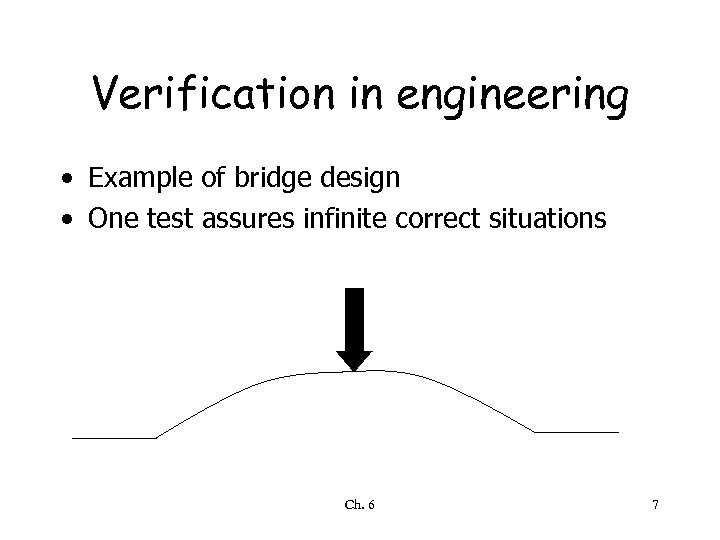Verification in engineering • Example of bridge design • One test assures infinite correct situations Ch. 6 7

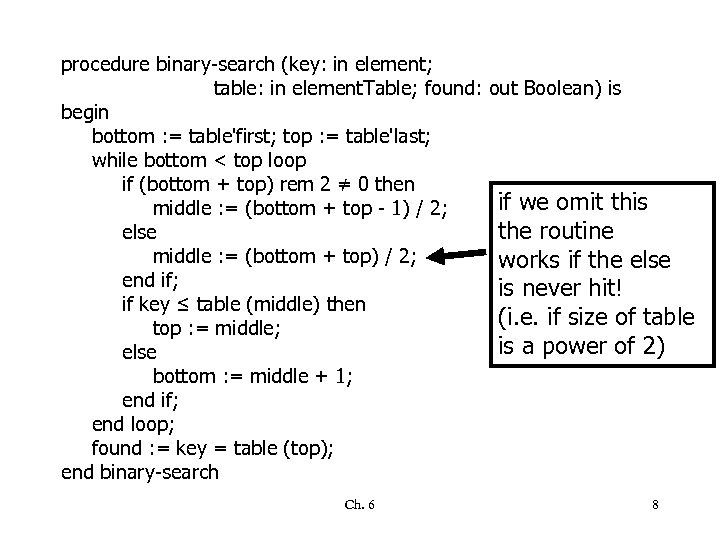procedure binary-search (key: in element; table: in element. Table; found: out Boolean) is begin bottom : = table'first; top : = table'last; while bottom < top loop if (bottom + top) rem 2 ≠ 0 then if we omit this middle : = (bottom + top - 1) / 2; the routine else middle : = (bottom + top) / 2; works if the else end if; is never hit! if key ≤ table (middle) then (i. e. if size of table top : = middle; is a power of 2) else bottom : = middle + 1; end if; end loop; found : = key = table (top); end binary-search Ch. 6 8

Goals of testing • To show the presence of bugs (Dijkstra, 1987) • If tests do detect failures, we cannot conclude that software is defect-free • Still, we need to do testing – driven by sound and systematic principles Ch. 6 9

Goals of testing (cont. ) • Should help isolate errors – to facilitate debugging • Should be repeatable – repeating the same experiment, we should get the same results • this may not be true because of the effect of execution environment on testing • because of nondeterminism • Should be accurate Ch. 6 10

Theoretical foundations of testing Ch. 6 11

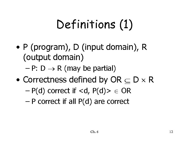Definitions (1) • P (program), D (input domain), R (output domain) – P: D R (may be partial) • Correctness defined by OR D R – P(d) correct if OR – P correct if all P(d) are correct Ch. 6 12

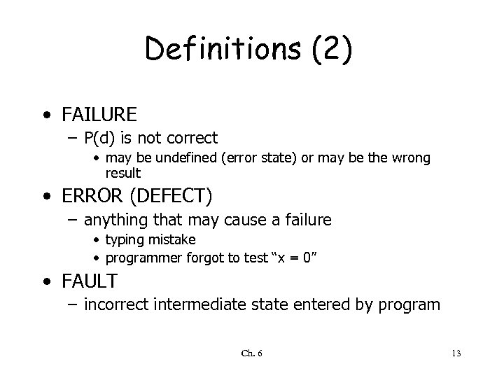Definitions (2) • FAILURE – P(d) is not correct • may be undefined (error state) or may be the wrong result • ERROR (DEFECT) – anything that may cause a failure • typing mistake • programmer forgot to test “x = 0” • FAULT – incorrect intermediate state entered by program Ch. 6 13

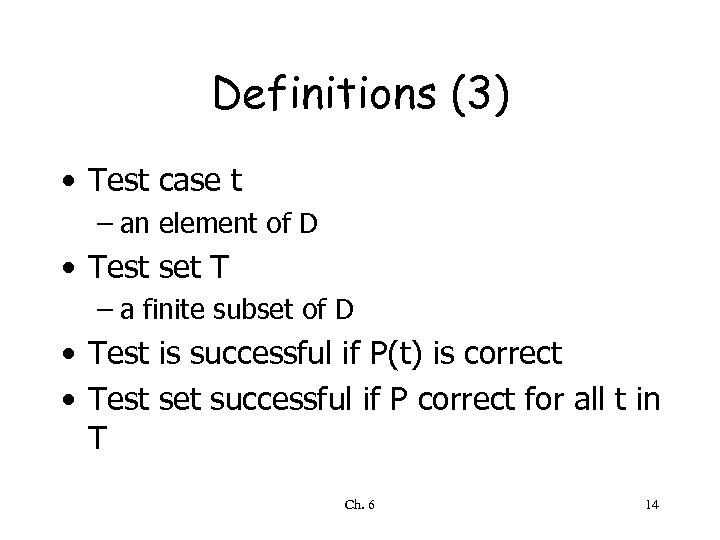Definitions (3) • Test case t – an element of D • Test set T – a finite subset of D • Test is successful if P(t) is correct • Test set successful if P correct for all t in T Ch. 6 14

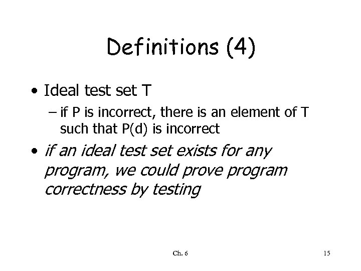Definitions (4) • Ideal test set T – if P is incorrect, there is an element of T such that P(d) is incorrect • if an ideal test set exists for any program, we could prove program correctness by testing Ch. 6 15

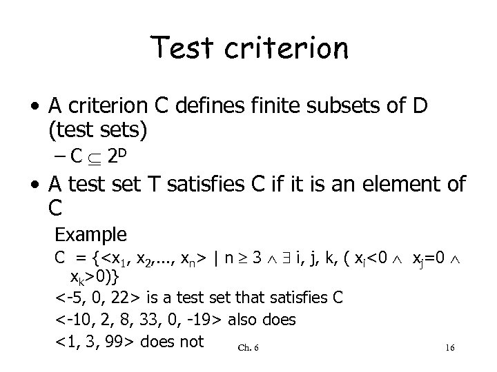Test criterion • A criterion C defines finite subsets of D (test sets) – C 2 D • A test set T satisfies C if it is an element of C Example C = { | n 3 i, j, k, ( xi<0 xj=0 xk>0)} <-5, 0, 22> is a test set that satisfies C <-10, 2, 8, 33, 0, -19> also does <1, 3, 99> does not Ch. 6 16

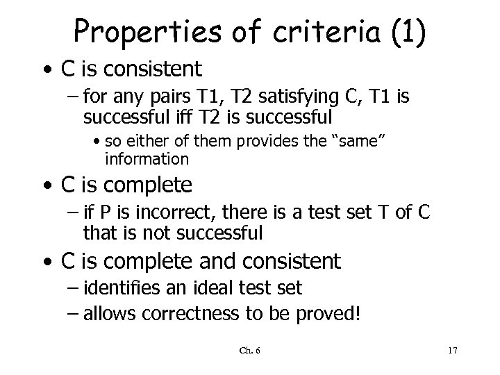Properties of criteria (1) • C is consistent – for any pairs T 1, T 2 satisfying C, T 1 is successful iff T 2 is successful • so either of them provides the “same” information • C is complete – if P is incorrect, there is a test set T of C that is not successful • C is complete and consistent – identifies an ideal test set – allows correctness to be proved! Ch. 6 17

Properties of criteria (2) • C 1 is finer than C 2 – for any program P • for any T 1 satisfying C 1 there is a subset T 2 of T 1 which satisfies C 2 Ch. 6 18

Properties of definitions • None is effective, i. e. , no algorithms exist to state if a program, test set, or criterion has that property • In particular, there is no algorithm to derive a test set that would prove program correctness – there is no constructive criterion that is consistent and complete Ch. 6 19

Empirical testing principles • Attempted compromise between the impossible and the inadequate • Find strategy to select significant test cases – significant=has high potential of uncovering presence of error Ch. 6 20

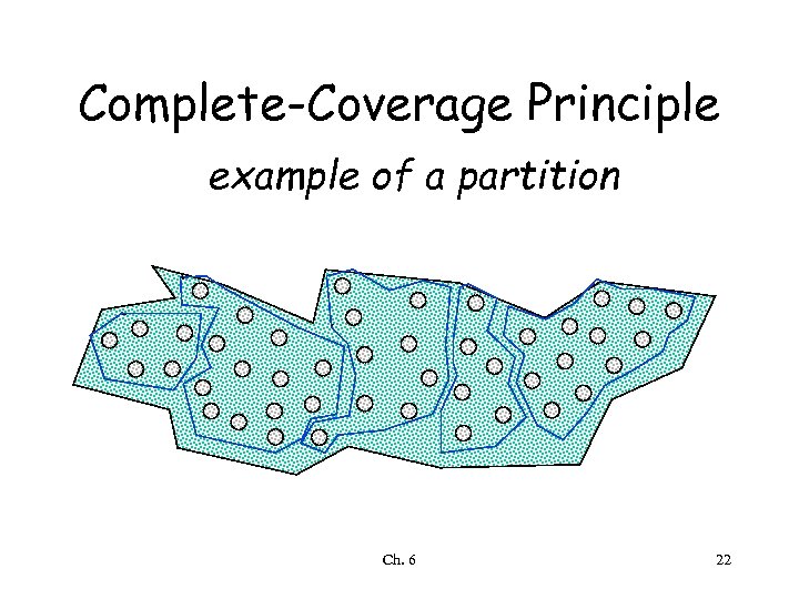
Complete-Coverage Principle • Try to group elements of D into subdomains D 1, D 2, …, Dn where any element of each Di is likely to have similar behavior – D = D 1 D 2 … Dn • Select one test as a representative of the subdomain • If Dj Dk for all j, k (partition), any element can be chosen from each subdomain • Otherwise choose representatives to minimize number of tests, yet fulfilling the principle Ch. 6 21

Complete-Coverage Principle example of a partition Ch. 6 22

Testing in the small We test individual modules • BLACK BOX (functional) testing – partitioning criteria based on the module’s specification – tests what the program is supposed to do • WHITE BOX (structural) testing – partitioning criteria based on module’s internal code – tests what the program does Ch. 6 23

White box testing derives test cases from program code Ch. 6 24

Structural Coverage Testing • (In)adequacy criteria – If significant parts of program structure are not tested, testing is inadequate • Control flow coverage criteria – Statement coverage – Edge coverage – Condition coverage – Path coverage Ch. 6 25

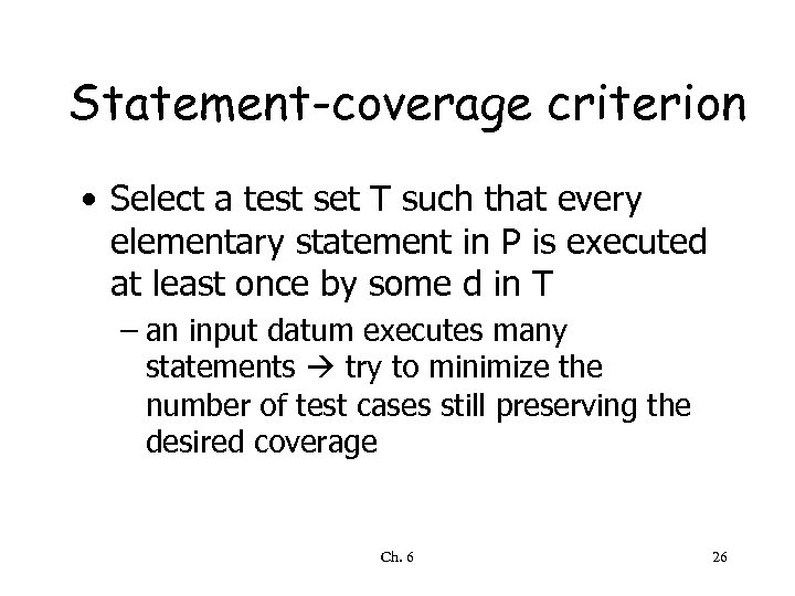Statement-coverage criterion • Select a test set T such that every elementary statement in P is executed at least once by some d in T – an input datum executes many statements try to minimize the number of test cases still preserving the desired coverage Ch. 6 26

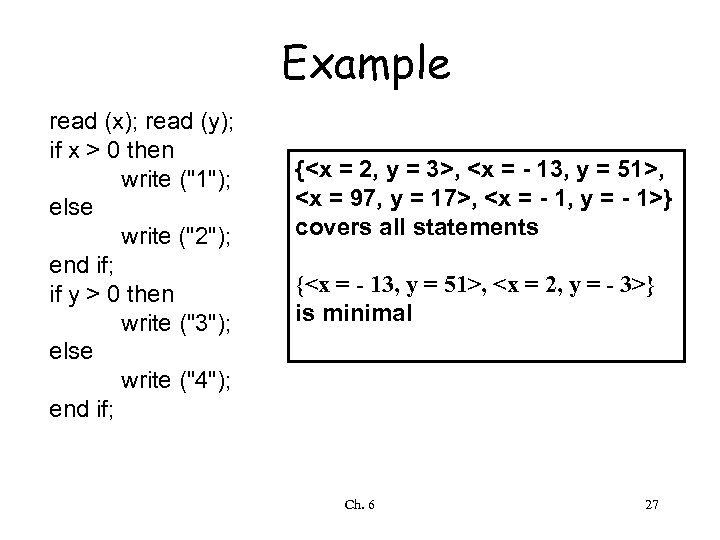Example read (x); read (y); if x > 0 then write ("1"); else write ("2"); end if; if y > 0 then write ("3"); else write ("4"); end if; {, , , } covers all statements {, } is minimal Ch. 6 27

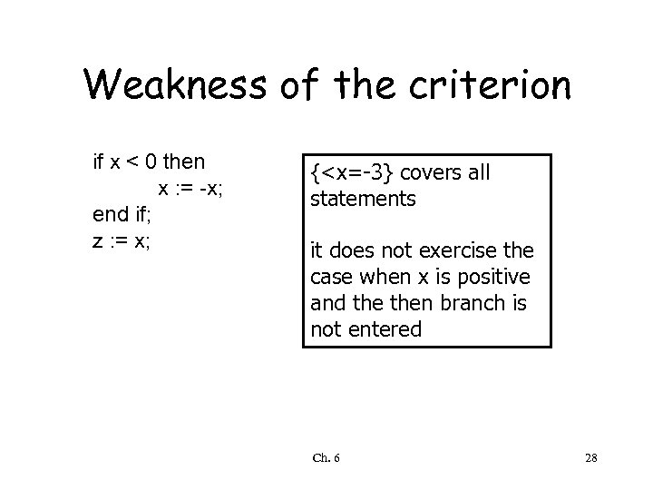Weakness of the criterion if x < 0 then x : = -x; end if; z : = x; {

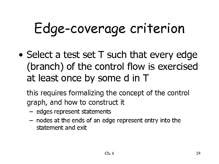Edge-coverage criterion • Select a test set T such that every edge (branch) of the control flow is exercised at least once by some d in T this requires formalizing the concept of the control graph, and how to construct it – edges represent statements – nodes at the ends of an edge represent entry into the statement and exit Ch. 6 29

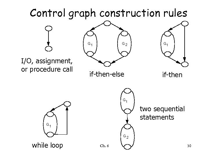Control graph construction rules G 1 I/O, assignment, or procedure call G 2 if-then-else G 1 if-then G 1 two sequential statements G 1 G 2 while loop Ch. 6 30

Simplification a sequence of edges can be collapsed into just one edge Ch. 6 31

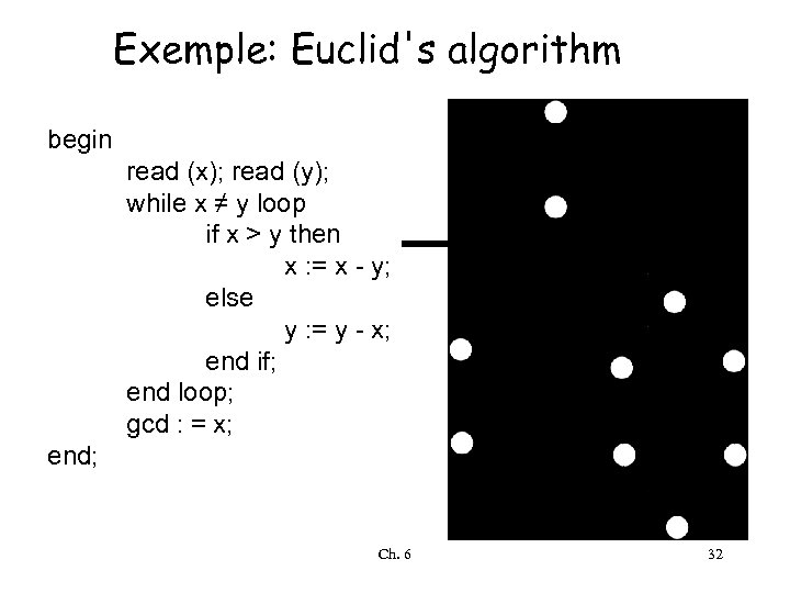Exemple: Euclid's algorithm begin read (x); read (y); while x ≠ y loop if x > y then x : = x - y; else y : = y - x; end if; end loop; gcd : = x; end; Ch. 6 32

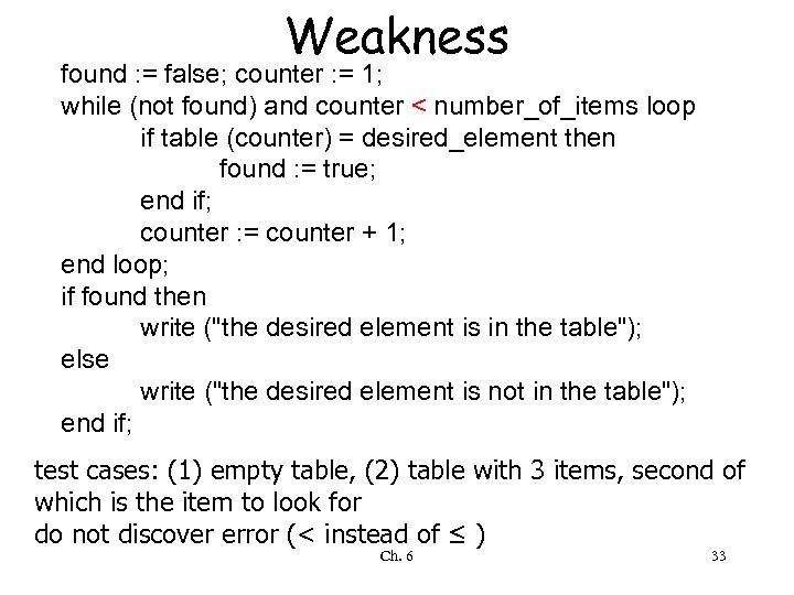Weakness found : = false; counter : = 1; while (not found) and counter < number_of_items loop if table (counter) = desired_element then found : = true; end if; counter : = counter + 1; end loop; if found then write ("the desired element is in the table"); else write ("the desired element is not in the table"); end if; test cases: (1) empty table, (2) table with 3 items, second of which is the item to look for do not discover error (< instead of ≤ ) Ch. 6 33

Condition-coverage criterion • Select a test set T such that every edge of P’s control flow is traversed and all possible values of the constituents of compound conditions are exercised at least once – it is finer than edge coverage Ch. 6 34

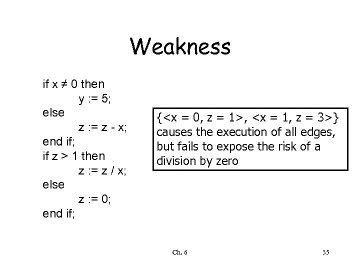Weakness if x ≠ 0 then y : = 5; else z : = z - x; end if; if z > 1 then z : = z / x; else z : = 0; end if; {, } causes the execution of all edges, but fails to expose the risk of a division by zero Ch. 6 35

Path-coverage criterion • Select a test set T which traverses all paths from the initial to the final node of P’s control flow – it is finer than previous kinds of coverage – however, number of paths may be too large, or even infinite (see while loops) • additional constraints must be provided Ch. 6 36

The infeasibility problem • Syntactically indicated behaviors (statements, edges, etc. ) are often impossible – unreachable code, infeasible edges, paths, etc. • Adequacy criteria may be impossible to satisfy – manual justification for omitting each impossible test case – adequacy “scores” based on coverage • example: 95% statement coverage Ch. 6 37

Further problem • What if the code omits the implementation of some part of the specification? • White box test cases derived from the code will ignore that part of the specification! Ch. 6 38

Black box testing derives test cases from specifications Ch. 6 39

The specification The program receives as input a record describing an invoice. (A detailed description of the format of the record is given. ) The invoice must be inserted into a file of invoices that is sorted by date. The invoice must be inserted in the appropriate position: If other invoices exist in the file with the same date, then the invoice should be inserted after the last one. Also, some consistency checks must be performed: The program should verify whether the customer is already in a corresponding file of customers, whether the customer’s data in the two files match, etc. Ch. 6 40

Did you consider these cases? • An invoice whose date is the current date • An invoice whose date is before the current date (This might be even forbidden by law) This case, in turn, can be split into the two following subcases: • An invoice whose date is the same as that some existing invoice • An invoice whose date does not exist in any previously recorded invoice • Several incorrect invoices, checking different types of inconsistencies Ch. 6 41

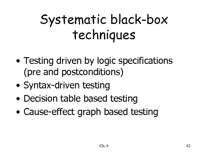Systematic black-box techniques • Testing driven by logic specifications (pre and postconditions) • Syntax-driven testing • Decision table based testing • Cause-effect graph based testing Ch. 6 42

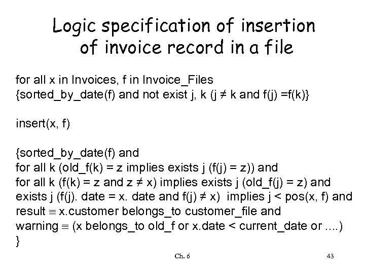Logic specification of insertion of invoice record in a file for all x in Invoices, f in Invoice_Files {sorted_by_date(f) and not exist j, k (j ≠ k and f(j) =f(k)} insert(x, f) {sorted_by_date(f) and for all k (old_f(k) = z implies exists j (f(j) = z)) and for all k (f(k) = z and z ≠ x) implies exists j (old_f(j) = z) and exists j (f(j). date = x. date and f(j) ≠ x) implies j < pos(x, f) and result º x. customer belongs_to customer_file and warning º (x belongs_to old_f or x. date < current_date or. . ) } Ch. 6 43

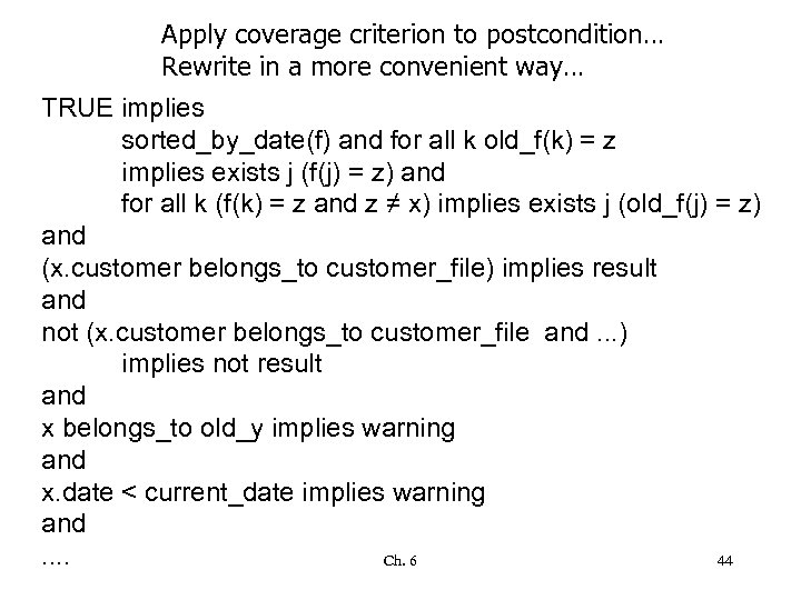Apply coverage criterion to postcondition… Rewrite in a more convenient way… TRUE implies sorted_by_date(f) and for all k old_f(k) = z implies exists j (f(j) = z) and for all k (f(k) = z and z ≠ x) implies exists j (old_f(j) = z) and (x. customer belongs_to customer_file) implies result and not (x. customer belongs_to customer_file and. . . ) implies not result and x belongs_to old_y implies warning and x. date < current_date implies warning and. . Ch. 6 44

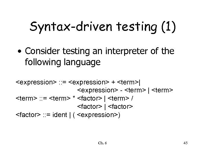Syntax-driven testing (1) • Consider testing an interpreter of the following language : : = + | - | : : = * | / | : : = ident | ( ) Ch. 6 45

Syntax-driven testing (2) • Apply complete coverage principle to all grammar rules • Generate a test case for each rule of the grammar – note, however that the test case might also cover other rules • Note: the specification is formal, and test generation can be automated Ch. 6 46

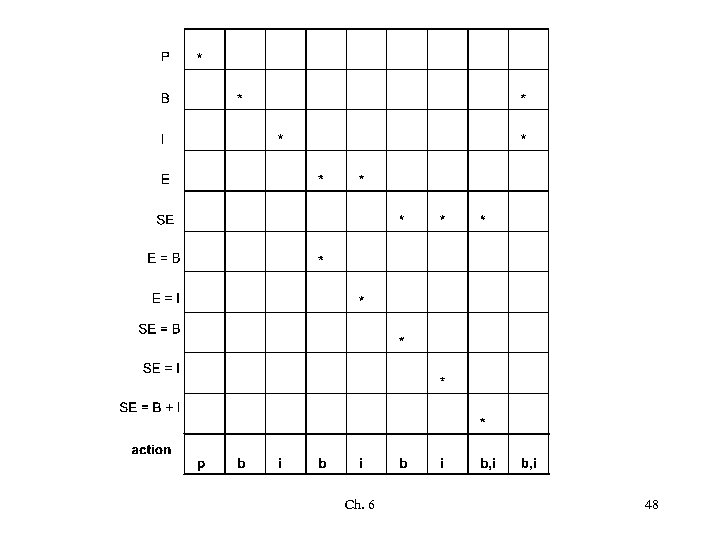
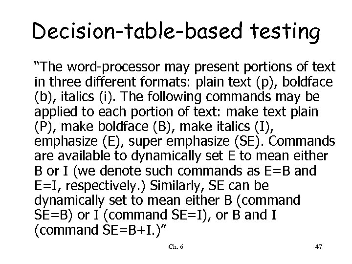Decision-table-based testing “The word-processor may present portions of text in three different formats: plain text (p), boldface (b), italics (i). The following commands may be applied to each portion of text: make text plain (P), make boldface (B), make italics (I), emphasize (E), super emphasize (SE). Commands are available to dynamically set E to mean either B or I (we denote such commands as E=B and E=I, respectively. ) Similarly, SE can be dynamically set to mean either B (command SE=B) or I (command SE=I), or B and I (command SE=B+I. )” Ch. 6 47

Ch. 6 48

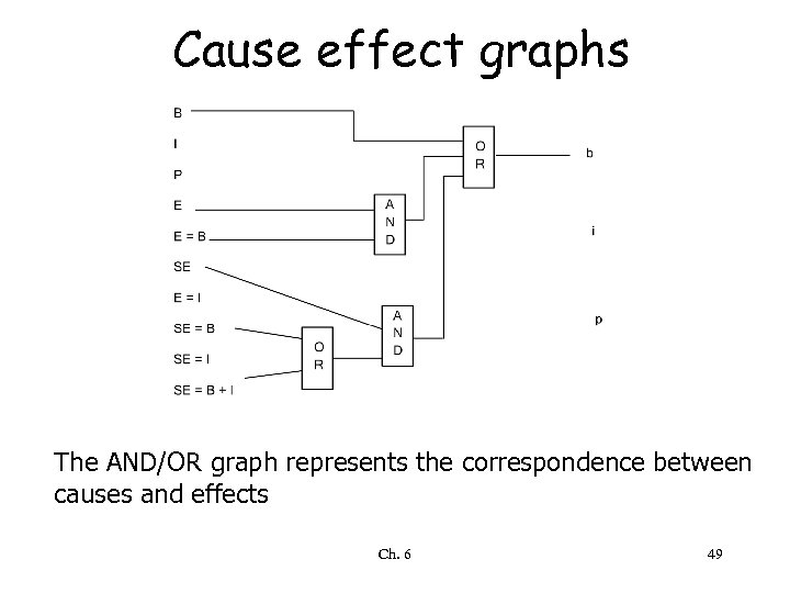Cause effect graphs The AND/OR graph represents the correspondence between causes and effects Ch. 6 49

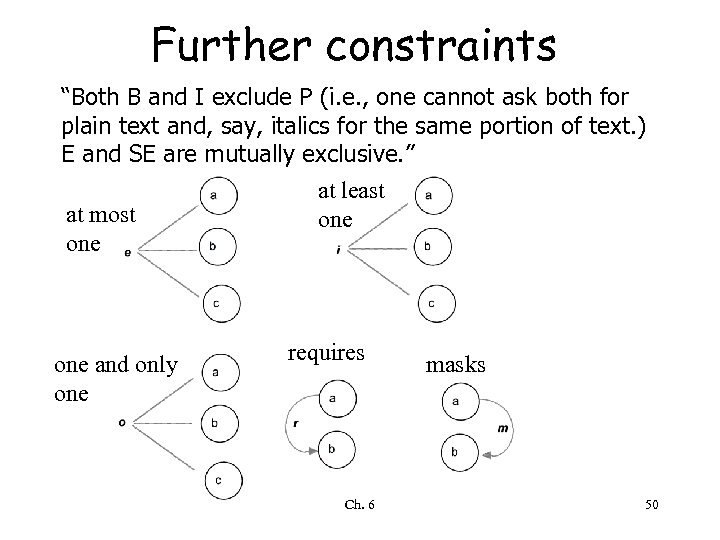Further constraints “Both B and I exclude P (i. e. , one cannot ask both for plain text and, say, italics for the same portion of text. ) E and SE are mutually exclusive. ” at least at most one one and only one requires Ch. 6 masks 50

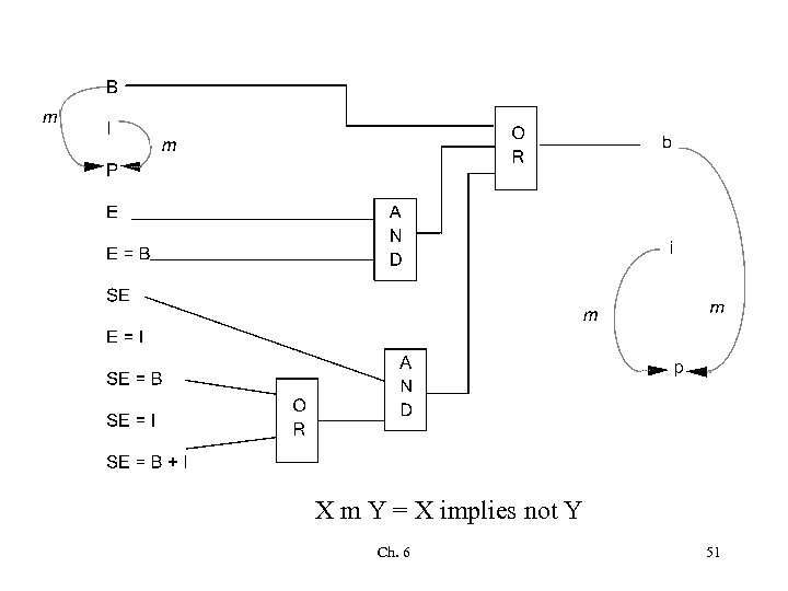X m Y = X implies not Y Ch. 6 51

Coverage criterion • Generate all possible input combinations and check outputs • May reduce the number by going backwards from outputs – OR node with true output: • use input combinations with only one true input – AND node with false output: • use input combinations with only one false input Ch. 6 52

Testing boundary conditions • Testing criteria partition input domain in classes, assuming that behavior is "similar" for all data within a class • Some typical programming errors, however, just happen to be at the boundary between different classes Ch. 6 53

Criterion • After partitioning the input domain D into several classes, test the program using input values not only “inside” the classes, but also at their boundaries • This applies to both white-box and black -box techniques Ch. 6 54

The oracle problem How to inspect the results of test executions to reveal failures • Oracles are required at each stage of testing • Automated test oracles are required for running large amounts of tests • Oracles are difficult to design - no universal recipe Ch. 6 55

Testing in the large • Module testing – testing a single module • Integration testing – integration of modules and subsystems • System testing – testing the entire system • Acceptance testing – performed by the customer Ch. 6 56

Module testing • Scaffolding needed to create the environment in which the module should be tested – stubs • modules used by the module under test – driver • module activating the module under test Ch. 6 57

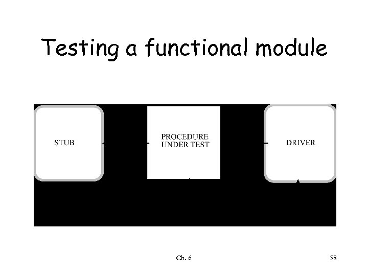Testing a functional module Ch. 6 58

Integration testing • Big-bang approach – first test individual modules in isolation – then test integrated system • Incremental approach – modules are progressively integrated and tested • can proceed both top-down and bottom-up according to the USES relation Ch. 6 59

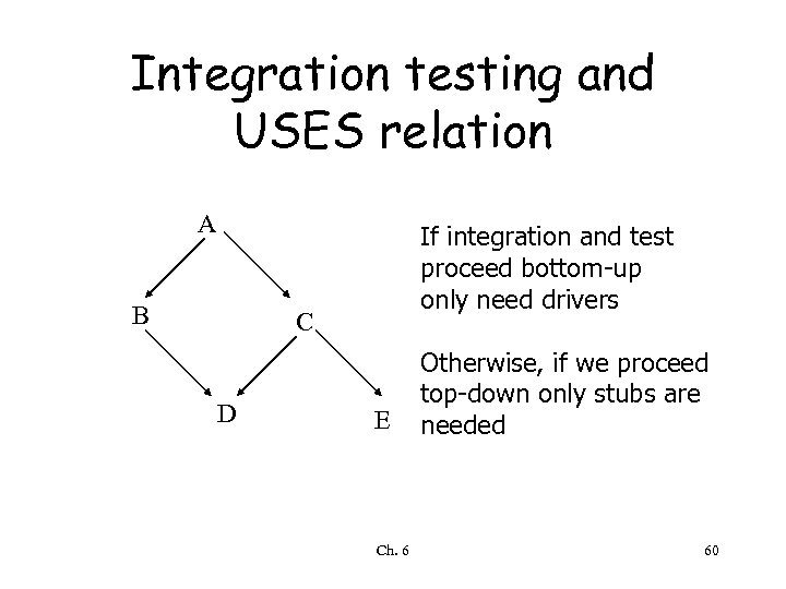Integration testing and USES relation A B If integration and test proceed bottom-up only need drivers C D E Ch. 6 Otherwise, if we proceed top-down only stubs are needed 60

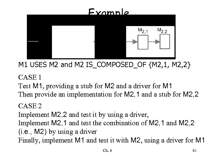Example M 1 USES M 2 and M 2 IS_COMPOSED_OF {M 2, 1, M 2, 2} CASE 1 Test M 1, providing a stub for M 2 and a driver for M 1 Then provide an implementation for M 2, 1 and a stub for M 2, 2 CASE 2 Implement M 2, 2 and test it by using a driver, Implement M 2, 1 and test the combination of M 2, 1 and M 2, 2 (i. e. , M 2) by using a driver Finally, implement M 1 and test it with M 2, using a driver for M 1 Ch. 6 61

Testing OO programs • New issues – inheritance – genericity – polymorphism – dynamic binding • Open problems still exist Ch. 6 62

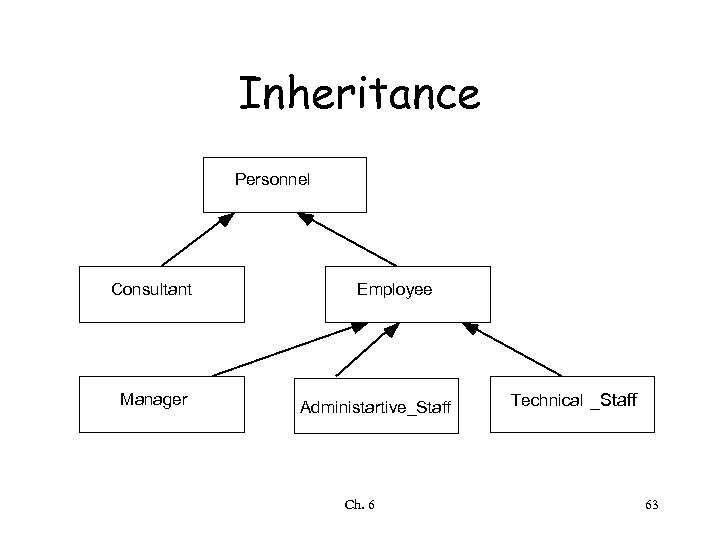Inheritance Personnel Consultant Manager Employee Administartive_Staff Ch. 6 Technical _Staff 63

How to test classes of the hierarchy? • “Flattening” the whole hierarchy and considering every class as a totally independent component – does not exploit incrementality • Finding an ad-hoc way to take advantage of the hierarchy Ch. 6 64

A sample strategy • A test that does not have to be repeated for any heir • A test that must be performed for heir class X and all of its further heirs • A test that must be redone by applying the same input data, but verifying that the output is not (or is) changed • A test that must be modified by adding other input parameters and verifying that the output changes accordingly Ch. 6 65

Separate concerns in testing • • Testing for functionality is not enough Overload testing Robustness testing Regression testing – organize testing with the purpose of verifying possible regressions of software during its life—that is, degradations of correctness or other qualities due to later modifications Ch. 6 66

Testing concurrent and realtime systems • Nondeterminism inherent in concurrency affects repeatability • For real-time systems, a test case consists not only of input data, but also of the times when such data are supplied Ch. 6 67

Analysis Ch. 6 68

Analysis vs. testing • Testing characterizes a single execution • Analysis characterizes a class of executions; it is based on a model • They have complementary advantages and disadvantages Ch. 6 69

Informal analysis techniques Code walkthroughs • Recommended prescriptions – Small number of people (three to five) – Participants receive written documentation from the designer a few days before the meeting – Predefined duration of meeting (a few hours) – Focus on the discovery of errors, not on fixing them – Participants: designer, moderator, and a secretary – Foster cooperation; no evaluation of people • Experience shows that most errors are discovered by the designer during the presentation, while trying to explain the design to other people. Ch. 6 70

Informal analysis techniques Code inspection • A reading technique aiming at error discovery • Based on checklists; e. g. : – use of uninitialized variables; – jumps into loops; – nonterminating loops; – array indexes out of bounds; –… Ch. 6 71

Correctness proofs Ch. 6 72

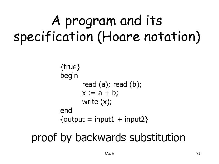A program and its specification (Hoare notation) {true} begin read (a); read (b); x : = a + b; write (x); end {output = input 1 + input 2} proof by backwards substitution Ch. 6 73

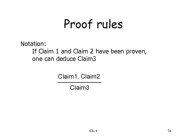Proof rules Notation: If Claim 1 and Claim 2 have been proven, one can deduce Claim 3 Claim 1, Claim 2 Claim 3 Ch. 6 74

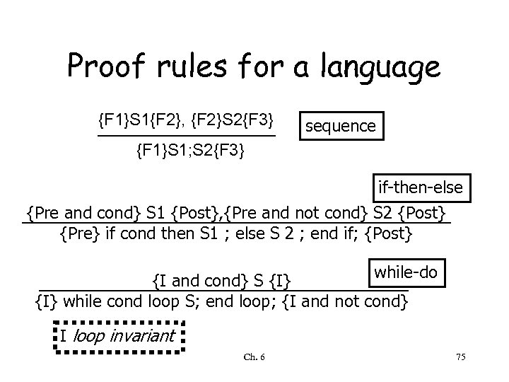Proof rules for a language {F 1}S 1{F 2}, {F 2}S 2{F 3} sequence {F 1}S 1; S 2{F 3} if-then-else {Pre and cond} S 1 {Post}, {Pre and not cond} S 2 {Post} {Pre} if cond then S 1 ; else S 2 ; end if; {Post} while-do {I and cond} S {I} while cond loop S; end loop; {I and not cond} I loop invariant Ch. 6 75

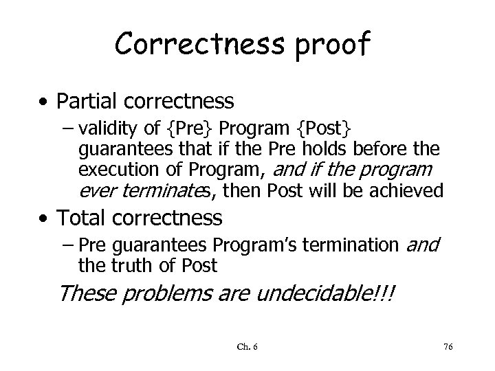Correctness proof • Partial correctness – validity of {Pre} Program {Post} guarantees that if the Pre holds before the execution of Program, and if the program ever terminates, then Post will be achieved • Total correctness – Pre guarantees Program’s termination and the truth of Post These problems are undecidable!!! Ch. 6 76

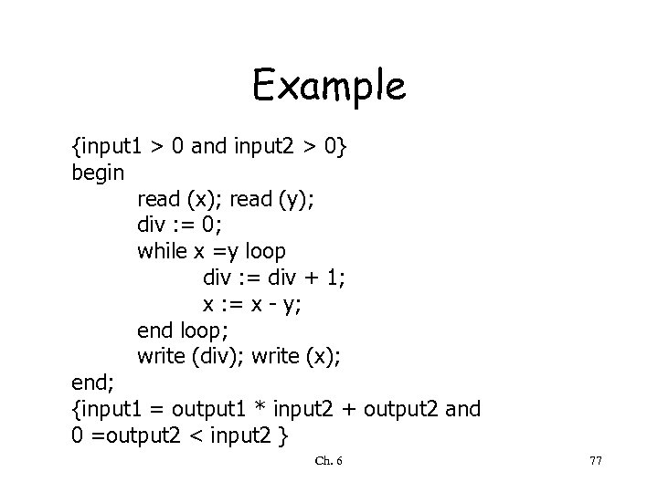Example {input 1 > 0 and input 2 > 0} begin read (x); read (y); div : = 0; while x =y loop div : = div + 1; x : = x - y; end loop; write (div); write (x); end; {input 1 = output 1 * input 2 + output 2 and 0 =output 2 < input 2 } Ch. 6 77

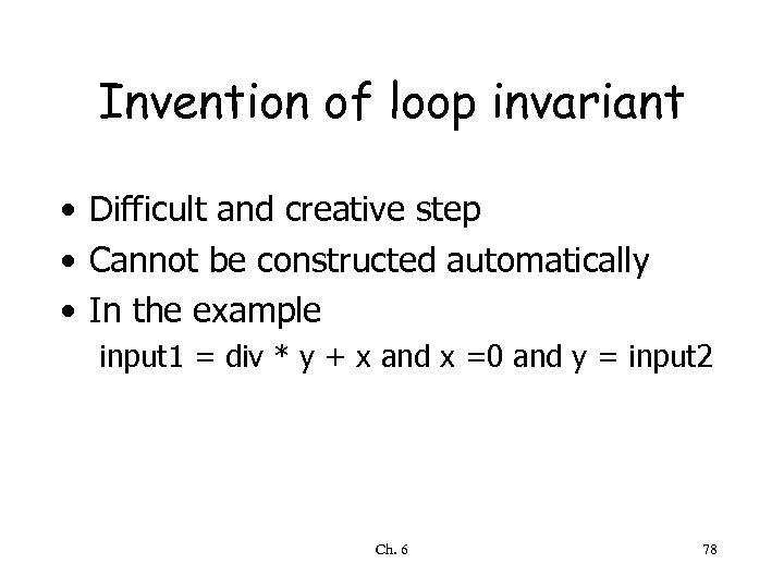Invention of loop invariant • Difficult and creative step • Cannot be constructed automatically • In the example input 1 = div * y + x and x =0 and y = input 2 Ch. 6 78

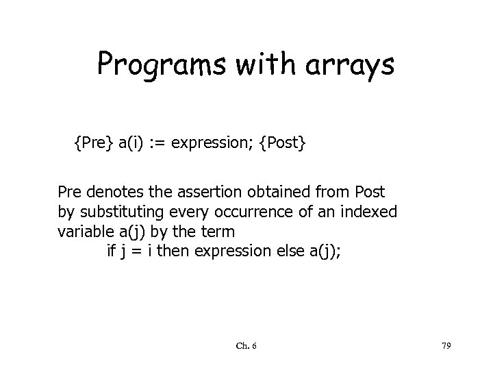Programs with arrays {Pre} a(i) : = expression; {Post} Pre denotes the assertion obtained from Post by substituting every occurrence of an indexed variable a(j) by the term if j = i then expression else a(j); Ch. 6 79

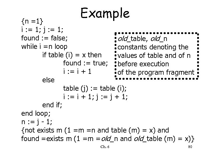Example {n =1} i : = 1; j : = 1; found : = false; old_table, old_n while i =n loop constants denoting the if table (i) = x then values of table and of n found : = true; before execution i : = i + 1 of the program fragment else table (j) : = table (i); i : = i + 1; j : = j + 1; end if; end loop; n : = j - 1; {not exists m (1 =m =n and table (m) = x) and found =exists m (1 =m =old_n and old_table (m) = x)} Ch. 6 80

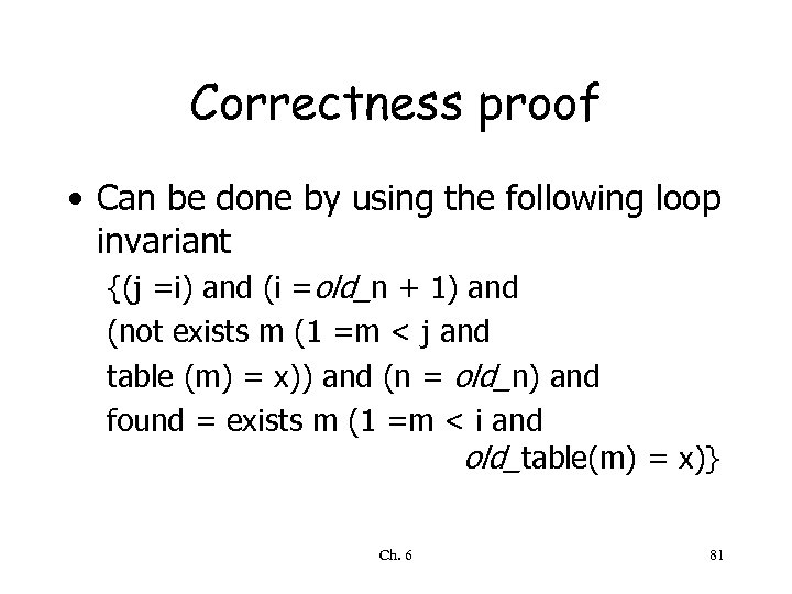Correctness proof • Can be done by using the following loop invariant {(j =i) and (i =old_n + 1) and (not exists m (1 =m < j and table (m) = x)) and (n = old_n) and found = exists m (1 =m < i and old_table(m) = x)} Ch. 6 81

Correctness proofs in the large • We can prove correctness of operations (e. g. , operations on an abstract data type) • Then use the result of the proof in proving fragments that operate on objects of the ADT Ch. 6 82

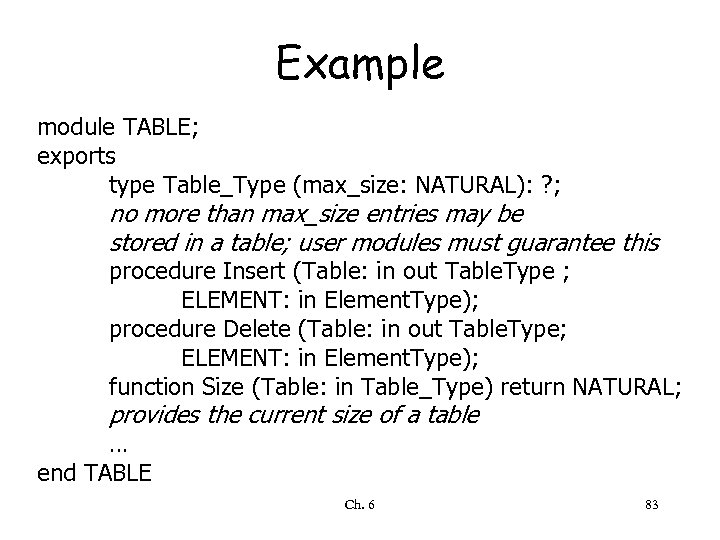Example module TABLE; exports type Table_Type (max_size: NATURAL): ? ; no more than max_size entries may be stored in a table; user modules must guarantee this procedure Insert (Table: in out Table. Type ; ELEMENT: in Element. Type); procedure Delete (Table: in out Table. Type; ELEMENT: in Element. Type); function Size (Table: in Table_Type) return NATURAL; provides the current size of a table … end TABLE Ch. 6 83

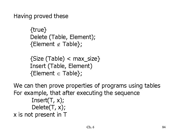Having proved these {true} Delete (Table, Element); {Element Table}; {Size (Table) < max_size} Insert (Table, Element) {Element Table}; We can then prove properties of programs using tables For example, that after executing the sequence Insert(T, x); Delete(T, x); x is not present in T Ch. 6 84

An assessment of correctness proofs • Still not used in practice • However – may be used for very critical portions – assertions may be the basis for a systematic way of inserting runtime checks – proofs may become more practical as more powerful support tools are developed – knowledge of correctness theory helps programmers being rigorous Ch. 6 85

Symbolic execution • Can be viewed as a middle way between testing and analysis • Executes the program on symbolic values • One symbolic execution corresponds to many actual executions Ch. 6 86

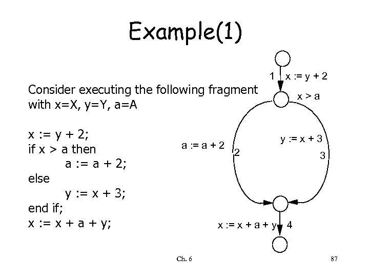Example(1) Consider executing the following fragment with x=X, y=Y, a=A x : = y + 2; if x > a then a : = a + 2; else y : = x + 3; end if; x : = x + a + y; a : = a + 2 1 x > a y : = x + 3 2 x : = x + a + y Ch. 6 x : = y + 2 3 4 87

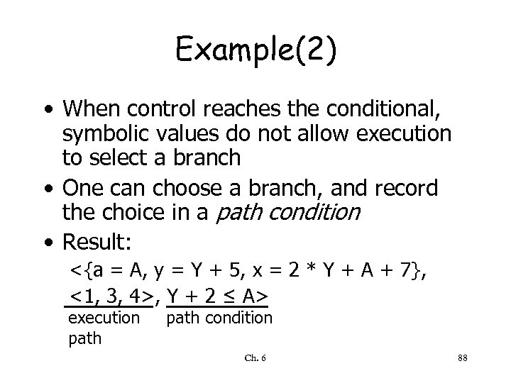Example(2) • When control reaches the conditional, symbolic values do not allow execution to select a branch • One can choose a branch, and record the choice in a path condition • Result: <{a = A, y = Y + 5, x = 2 * Y + A + 7}, <1, 3, 4>, Y + 2 ≤ A> execution path condition Ch. 6 88

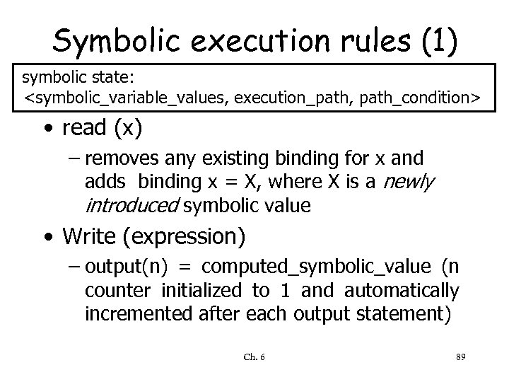Symbolic execution rules (1) symbolic state: • read (x) – removes any existing binding for x and adds binding x = X, where X is a newly introduced symbolic value • Write (expression) – output(n) = computed_symbolic_value (n counter initialized to 1 and automatically incremented after each output statement) Ch. 6 89

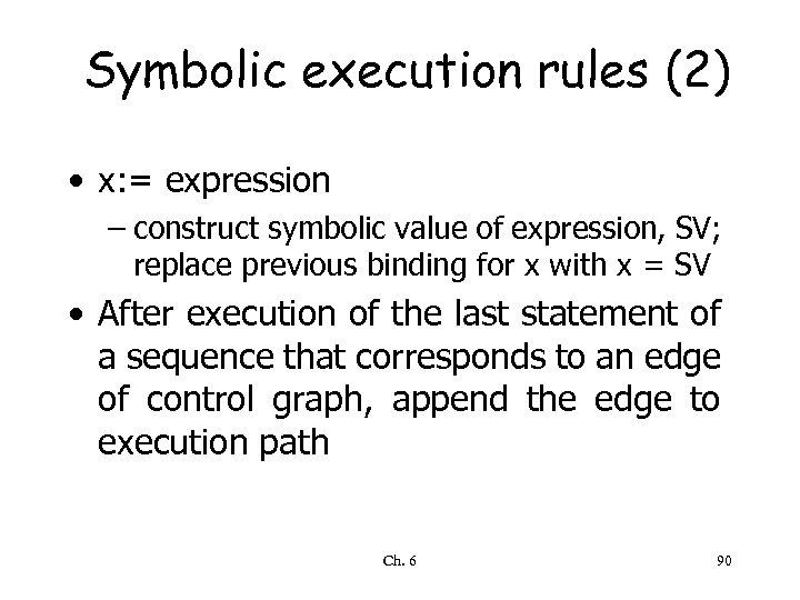Symbolic execution rules (2) • x: = expression – construct symbolic value of expression, SV; replace previous binding for x with x = SV • After execution of the last statement of a sequence that corresponds to an edge of control graph, append the edge to execution path Ch. 6 90

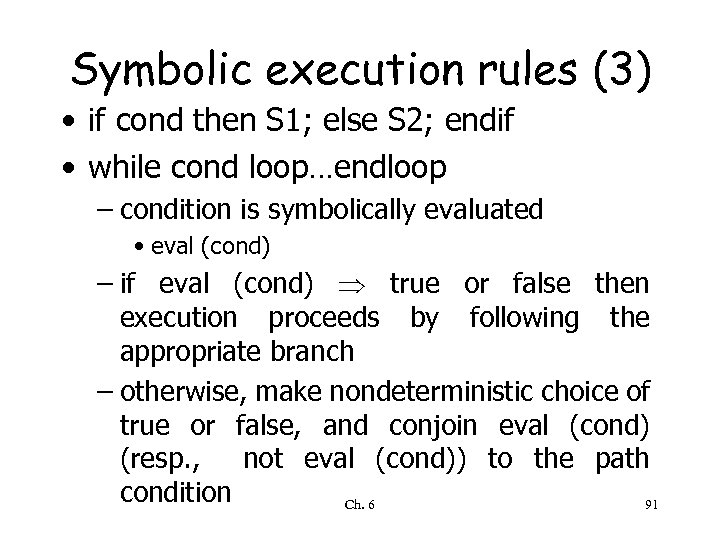Symbolic execution rules (3) • if cond then S 1; else S 2; endif • while cond loop…endloop – condition is symbolically evaluated • eval (cond) – if eval (cond) true or false then execution proceeds by following the appropriate branch – otherwise, make nondeterministic choice of true or false, and conjoin eval (cond) (resp. , not eval (cond)) to the path condition Ch. 6 91

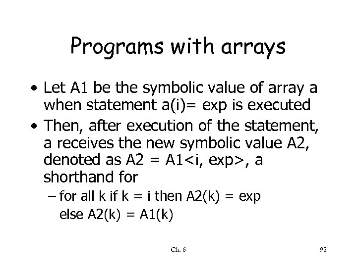Programs with arrays • Let A 1 be the symbolic value of array a when statement a(i)= exp is executed • Then, after execution of the statement, a receives the new symbolic value A 2, denoted as A 2 = A 1, a shorthand for – for all k if k = i then A 2(k) = exp else A 2(k) = A 1(k) Ch. 6 92

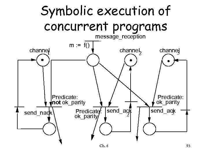Symbolic execution of concurrent programs message_reception m : = f() channel 1 channel 2 Predicate: not ok_parity send_nack channel 3 Predicate: ok_parity Predicate: send_ack 2 ok_parity Ch. 6 send_ack 3 93

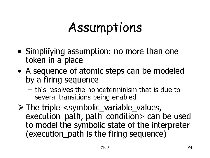Assumptions • Simplifying assumption: no more than one token in a place • A sequence of atomic steps can be modeled by a firing sequence – this resolves the nondeterminism that is due to several transitions being enabled Ø The triple can be used to model the symbolic state of the interpreter (execution_path is the firing sequence) Ch. 6 94

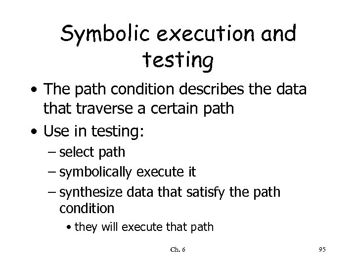Symbolic execution and testing • The path condition describes the data that traverse a certain path • Use in testing: – select path – symbolically execute it – synthesize data that satisfy the path condition • they will execute that path Ch. 6 95

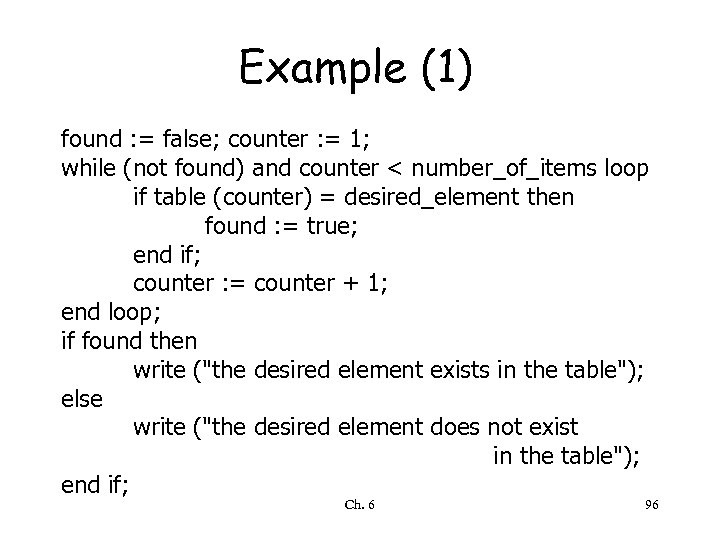Example (1) found : = false; counter : = 1; while (not found) and counter < number_of_items loop if table (counter) = desired_element then found : = true; end if; counter : = counter + 1; end loop; if found then write ("the desired element exists in the table"); else write ("the desired element does not exist in the table"); end if; Ch. 6 96

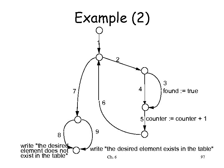Example (2) 1 2 4 7 3 found : = true 6 5 counter : = counter + 1 8 write "the desired element does not exist in the table" 9 write "the desired element exists in the table" Ch. 6 97

Model checking • Correctness verification, in general, is an undecidable problem • Model checking is a rather recent verification technique based on the fact that most interesting system properties become decidable (i. e. , algorithmically verifiable) when the system is modeled as a finite state machine Ch. 6 98

Principles • Describe a given system—software or otherwise—as an FSM • Express a given property of interest as a suitable formula • Verify whether the system’s behavior does indeed satisfy the desired property – this step can be performed automatically – the model checker either provides a proof that the property holds or gives a counterexample in the form of a test case that exposes the system’s failure to behave according to the property Ch. 6 99

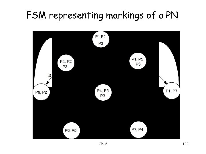FSM representing markings of a PN Ch. 6 100

The original PN Ch. 6 101

Properties and proofs • Property to be verified given through a formula (in temporal logic) • In the example, one can prove – there is always a computation that allows the left process to enter the critical region – there is no guarantee that the left process accesses the shared resource unless it already owns it Ch. 6 102

Why so many approaches to testing and analysis? • • • Testing versus (correctness) analysis Formal versus informal techniques White-box versus black-box techniques Techniques in the small/large Fully automatic vs. semiautomatic techniques (for undecidable properties) • … view all these as complementary Ch. 6 103

Debugging • The activity of locating and correcting errors • It can start once a failure has been detected • The goal is closing up the gap between a fault and failure – memory dumps, watch points – intermediate assertions can help Ch. 6 104

Verifying other qualities Ch. 6 105

Performance • Worst case analysis – focus is on proving that the system response time is bounded by some function of the external requests vs. average behavior • Standard deviation • Analytical vs. experimental approaches Ch. 6 106

Reliability (1) • There approaches to measuring reliability on a probabilistic basis, as in other engineering fields • Unfortunately there are some difficulties with this approach • Independence of failures does not hold for software Ch. 6 107

Reliability (2) • Reliability is concerned with measuring the probability of the occurrence of failure • Meaningful parameters include: • average total number of failures observed at time t: AF(t) • failure intensity: FI(t)=AF'(t) • mean time to failure at time t: MTTF(t)=1/FI(t) • Time in the model can be execution or clock or calendar time Ch. 6 108

Basic reliability model • Assumes that the decrement per failure experienced (i. e. , the derivative with respect to the number of detected failures) of the failure intensity function is constant – i. e. , FI is a function of AF FI(AF) = FI 0 (1 - AF/AF∞) where FI 0 is the initial failure intensity and AF∞ is the total number of failures • The model is based on optimistic hypothesis that a decrease in failures is due to the fixing of the errors that were sources of failures Ch. 6 109

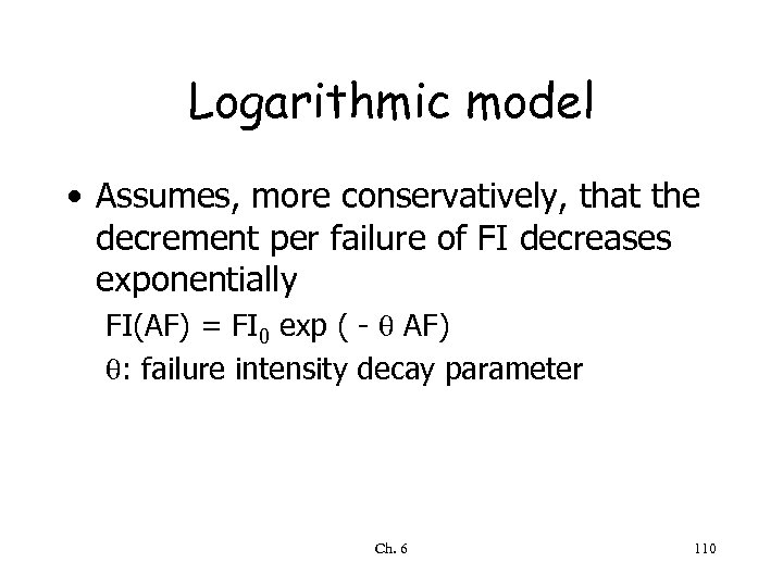Logarithmic model • Assumes, more conservatively, that the decrement per failure of FI decreases exponentially FI(AF) = FI 0 exp ( - AF) : failure intensity decay parameter Ch. 6 110

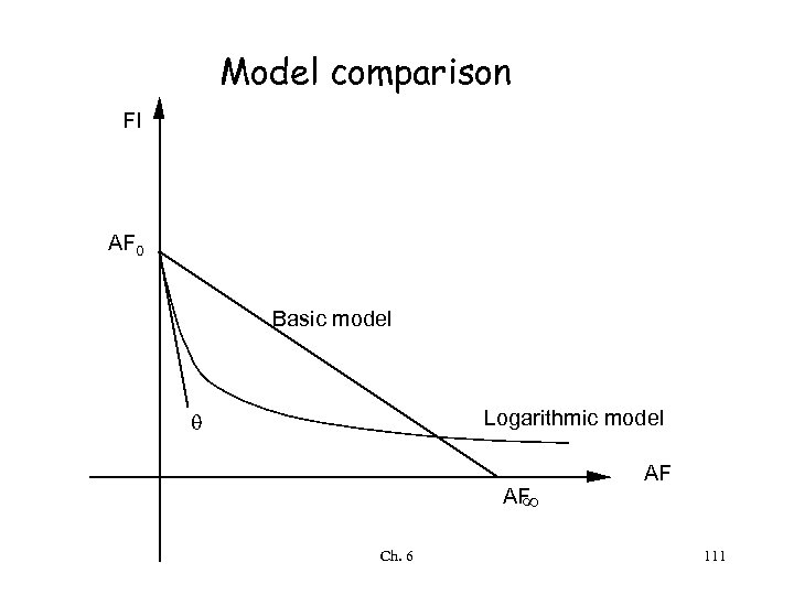Model comparison FI AF 0 Basic model Logarithmic model AF ¥ Ch. 6 AF 111

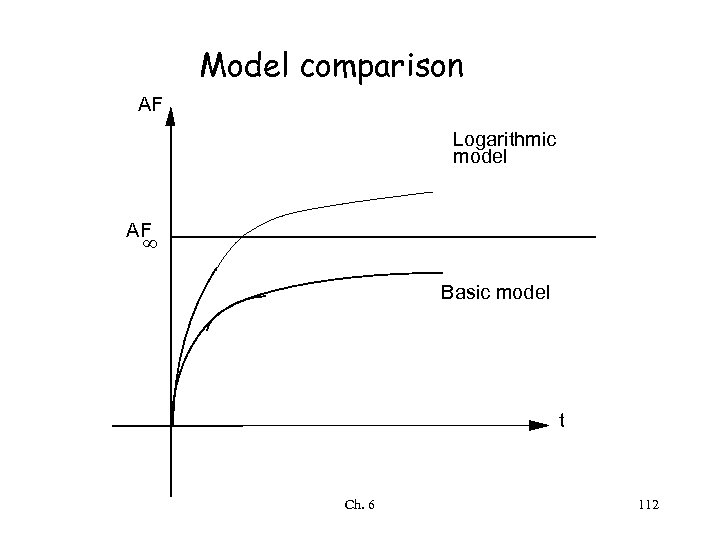Model comparison AF Logarithmic model AF ¥ Basic model t Ch. 6 112

Verifying subjective qualities • Consider notions like simplicity, reusability, understandability … • Software science (due to Halstead) has been an attempt Ch. 6 113

Halstead's software science • Tries to measure some software qualities, such as abstraction level, effort, … • by measuring some quantities on code, such as - h 1, number of distinct operators in the program - h 2, number of distinct operands in the program - N 1, number of occurrences of operators in the program - N 2, number of occurrences of operands in the program Ch. 6 114

Mc. Cabe's source code metric • Cyclomatic complexity of the control graph –C=e-n+2 p • e is # edges, n is # nodes, p is # connected components • Mc. Cabe contends that well-structured modules have C in range 3. . 7, and C = 10 is a reasonable upper limit for the complexity of a single module – confirmed by empirical evidence Ch. 6 115

Goal-question-metric (GQM) • Premise – software metrics must be used to analyze software qualities, not to evaluate people – quality evaluation must be of end product, intermediate products, and process – metrics must be defined in the context of a complete and well-designed quality improvement paradigm (QIP) Ch. 6 116

GQM • Not concerned with measuring a single quantity or group of quantities – e. g. , cyclomatic complexity • A method that is intended to lead from a precise definition of the objectives of measuring qualities (the goals) to the quantities (the metrics) whose measures are used to verify the achievement of such qualities. Ch. 6 117

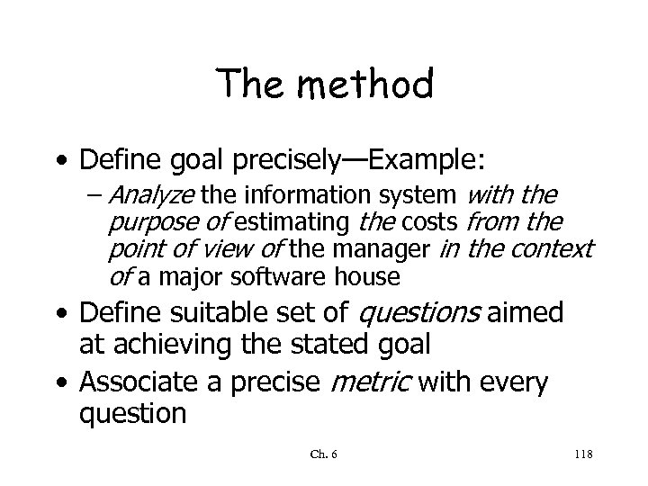The method • Define goal precisely—Example: – Analyze the information system with the purpose of estimating the costs from the point of view of the manager in the context of a major software house • Define suitable set of questions aimed at achieving the stated goal • Associate a precise metric with every question Ch. 6 118