c9e367941f6a9d37e01dbaf1ef91187d.ppt
- Количество слайдов: 66

Variation This presentation should be read by students at home to be able to solve problems

Home tasks 1. Task 5 should be sent to the formal leader of your group. 2. Home work you send to asidenko@fa. ru or to oknedis@bk. ru if any problems with the first email
Task 5 Part 1 • 1. Look thru tests from 1 -1 till 2 -47, pp. 721 from the test-book and note the numbers you are not sure you can answer properly. • 2. Look thru problems from number 1 till number 20, pp. 4 -11 from the problembook and note the numbers you are not sure you can solve properly. • 3. Send the report to the headman of your group
Home Work till March, 29 th, 1 a. m. • 1. Read textbooks, English “Variation” and Russian «Показатели вариации» presentations. • 2. Solve problems 134 (5 points), 152 (20), 160 (30), the max points for countdown - 80
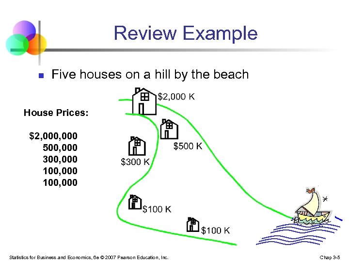
Review Example n Five houses on a hill by the beach House Prices: $2, 000 500, 000 300, 000 100, 000 Statistics for Business and Economics, 6 e © 2007 Pearson Education, Inc. Chap 3 -5
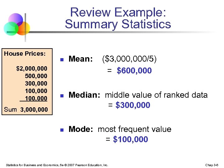
Review Example: Summary Statistics House Prices: $2, 000 500, 000 300, 000 100, 000 n n Sum 3, 000 n Mean: ($3, 000/5) = $600, 000 Median: middle value of ranked data = $300, 000 Mode: most frequent value = $100, 000 Statistics for Business and Economics, 6 e © 2007 Pearson Education, Inc. Chap 3 -6
Which measure of location is the “best”? n n Mean is generally used, unless extreme values (outliers) exist Then median is often used, since the median is not sensitive to extreme values. n Example: Median home prices may be reported for a region – less sensitive to outliers Statistics for Business and Economics, 6 e © 2007 Pearson Education, Inc. Chap 3 -7
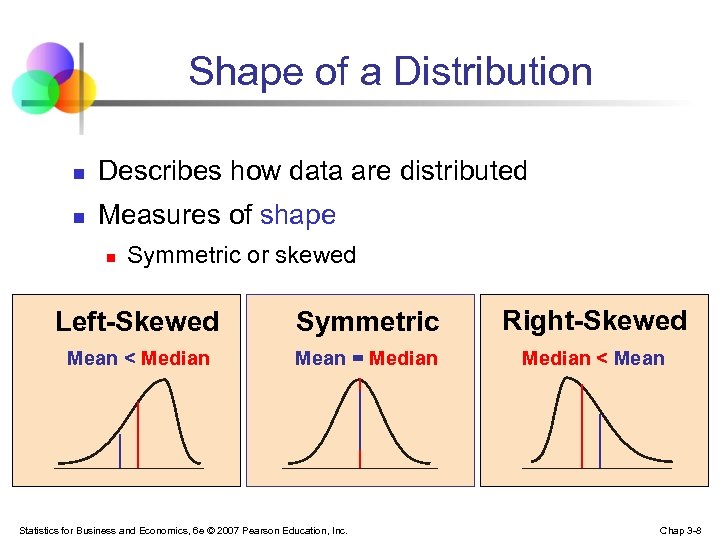
Shape of a Distribution n Describes how data are distributed n Measures of shape n Symmetric or skewed Left-Skewed Symmetric Right-Skewed Mean < Median Mean = Median < Mean Statistics for Business and Economics, 6 e © 2007 Pearson Education, Inc. Chap 3 -8
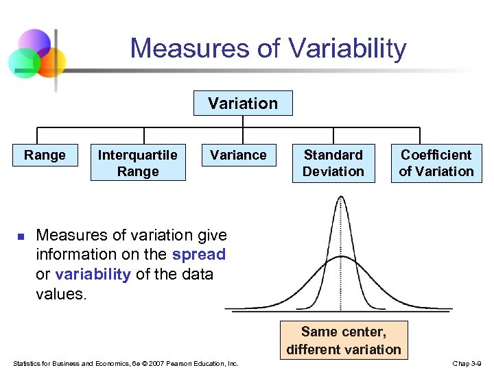
Measures of Variability Variation Range n Interquartile Range Variance Standard Deviation Coefficient of Variation Measures of variation give information on the spread or variability of the data values. Same center, different variation Statistics for Business and Economics, 6 e © 2007 Pearson Education, Inc. Chap 3 -9
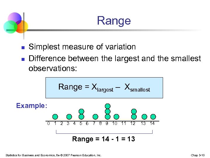
Range n n Simplest measure of variation Difference between the largest and the smallest observations: Range = Xlargest – Xsmallest Example: 0 1 2 3 4 5 6 7 8 9 10 11 12 13 14 Range = 14 - 1 = 13 Statistics for Business and Economics, 6 e © 2007 Pearson Education, Inc. Chap 3 -10
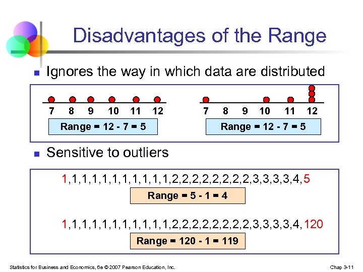
Disadvantages of the Range n Ignores the way in which data are distributed 7 8 9 10 11 12 Range = 12 - 7 = 5 n 7 8 9 10 11 12 Range = 12 - 7 = 5 Sensitive to outliers 1, 1, 1, 2, 2, 3, 3, 4, 5 Range = 5 - 1 = 4 1, 1, 1, 2, 2, 3, 3, 4, 120 Range = 120 - 1 = 119 Statistics for Business and Economics, 6 e © 2007 Pearson Education, Inc. Chap 3 -11
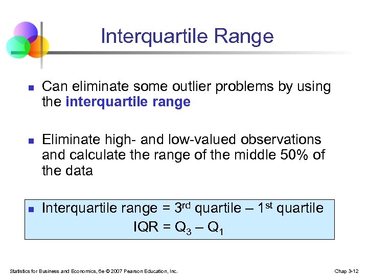
Interquartile Range n n n Can eliminate some outlier problems by using the interquartile range Eliminate high- and low-valued observations and calculate the range of the middle 50% of the data Interquartile range = 3 rd quartile – 1 st quartile IQR = Q 3 – Q 1 Statistics for Business and Economics, 6 e © 2007 Pearson Education, Inc. Chap 3 -12
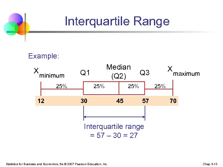
Interquartile Range Example: X minimum Q 1 25% 12 Median (Q 2) 25% 30 25% 45 X Q 3 maximum 25% 57 70 Interquartile range = 57 – 30 = 27 Statistics for Business and Economics, 6 e © 2007 Pearson Education, Inc. Chap 3 -13
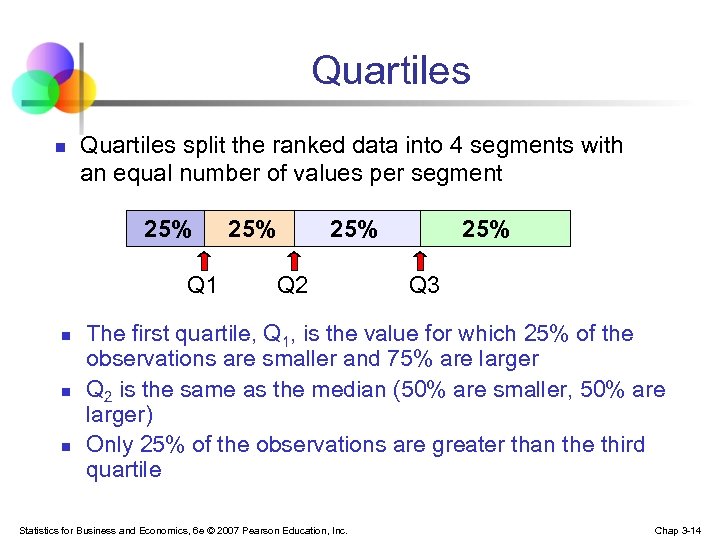
Quartiles n Quartiles split the ranked data into 4 segments with an equal number of values per segment 25% Q 1 n n n 25% Q 2 25% Q 3 The first quartile, Q 1, is the value for which 25% of the observations are smaller and 75% are larger Q 2 is the same as the median (50% are smaller, 50% are larger) Only 25% of the observations are greater than the third quartile Statistics for Business and Economics, 6 e © 2007 Pearson Education, Inc. Chap 3 -14
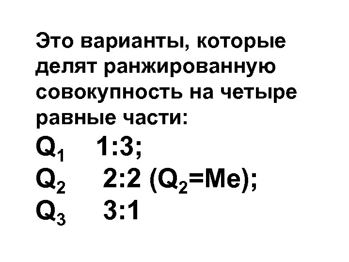
Это варианты, которые делят ранжированную совокупность на четыре равные части: Q 1 Q 2 Q 3 1: 3; 2: 2 (Q 2=Ме); 3: 1
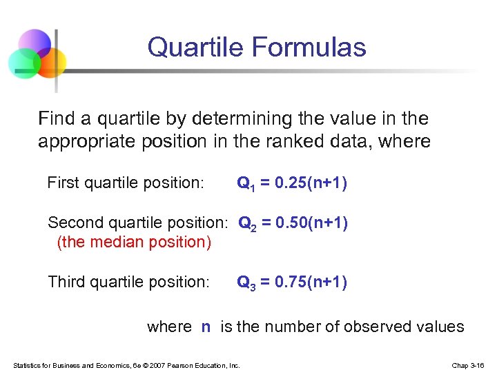
Quartile Formulas Find a quartile by determining the value in the appropriate position in the ranked data, where First quartile position: Q 1 = 0. 25(n+1) Second quartile position: Q 2 = 0. 50(n+1) (the median position) Third quartile position: Q 3 = 0. 75(n+1) where n is the number of observed values Statistics for Business and Economics, 6 e © 2007 Pearson Education, Inc. Chap 3 -16
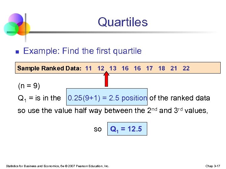
Quartiles n Example: Find the first quartile Sample Ranked Data: 11 12 13 16 16 17 18 21 22 (n = 9) Q 1 = is in the 0. 25(9+1) = 2. 5 position of the ranked data so use the value half way between the 2 nd and 3 rd values, so Statistics for Business and Economics, 6 e © 2007 Pearson Education, Inc. Q 1 = 12. 5 Chap 3 -17
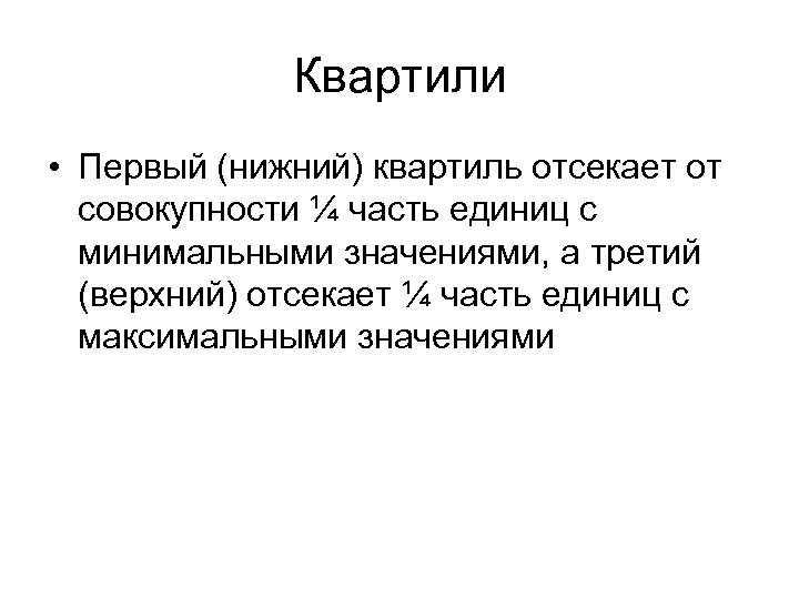
Квартили • Первый (нижний) квартиль отсекает от совокупности ¼ часть единиц с минимальными значениями, а третий (верхний) отсекает ¼ часть единиц с максимальными значениями
Квартили • Мы как бы отбрасываем нетипичные, случайные значения признака. С помощью квартилей мы определяем границы, где находятся 50% единиц, наиболее характерные для этой совокупности
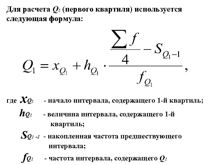
Для расчета Q 1 (первого квартиля) используется следующая формула: где x. Q h. Q 1 1 SQ f. Q 1 -1 1 - начало интервала, содержащего 1 -й квартиль; - величина интервала, содержащего 1 -й квартиль; - накопленная частота предшествующего интервала; - частота интервала, содержащего Q 1

Интервалом, содержащим Q 1, является тот интервал, для которого накопленная частота впервые превышает ¼ от суммы частот
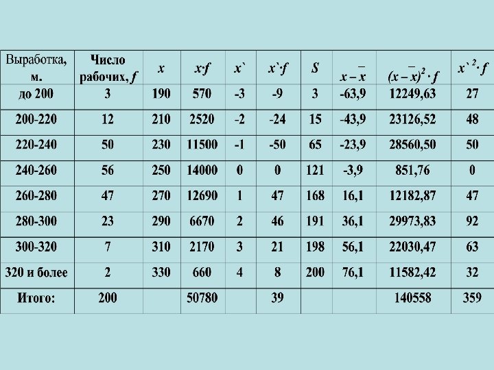
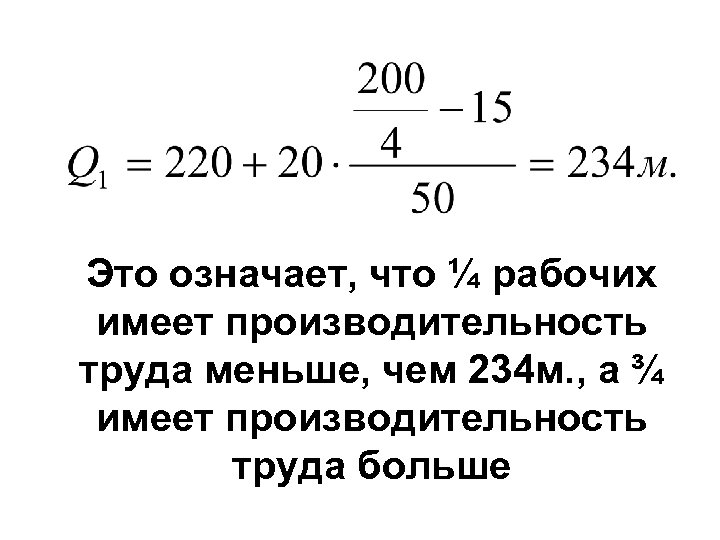
Это означает, что ¼ рабочих имеет производительность труда меньше, чем 234 м. , а ¾ имеет производительность труда больше
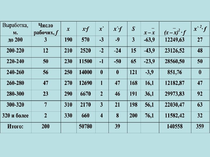
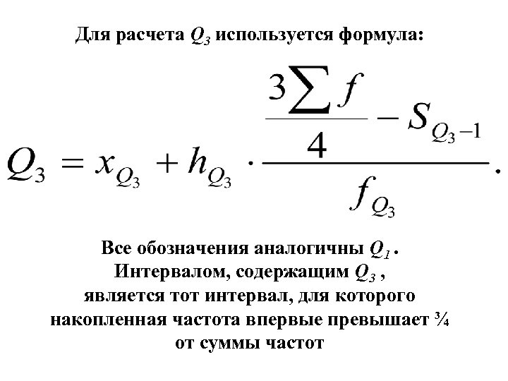
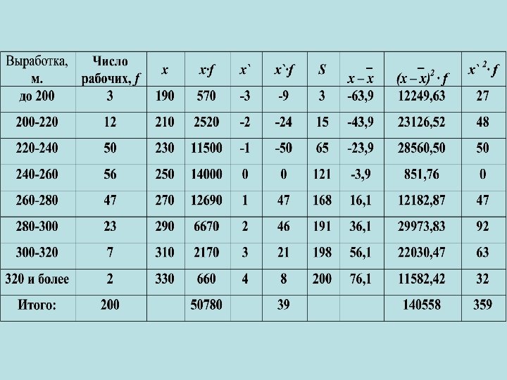
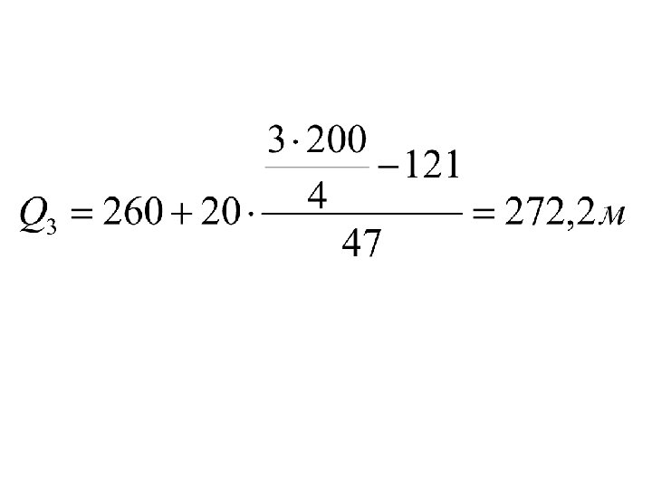
Для расчета Q 3 используется формула: Все обозначения аналогичны Q 1. Интервалом, содержащим Q 3 , является тот интервал, для которого накопленная частота впервые превышает ¾ от суммы частот

Децили это варианты, которые делят ранжированную совокупность на 10 равных частей
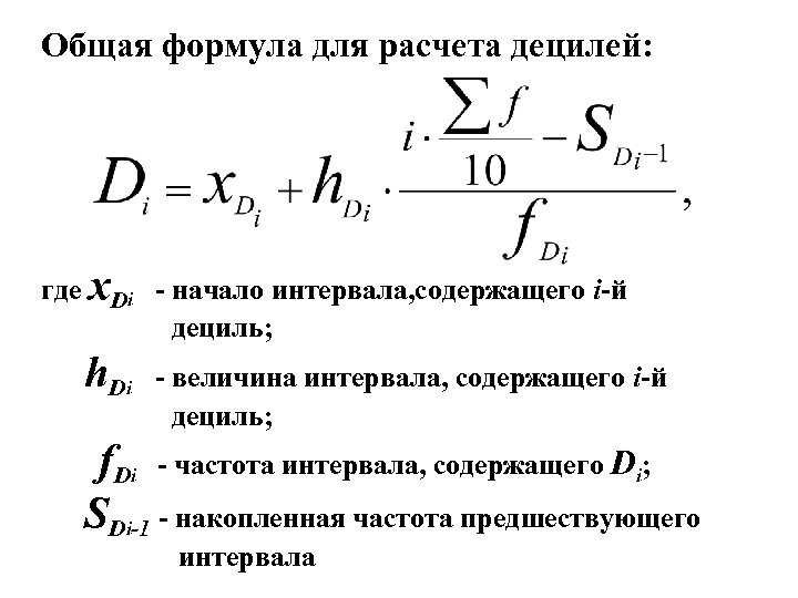
Общая формула для расчета децилей: где x. Di - начало интервала, содержащего i-й дециль; h Di - величина интервала, содержащего i-й дециль; f. Di - частота интервала, содержащего Di; SDi-1 - накопленная частота предшествующего интервала

Интервалом, содержащим Di , является тот интервал, для которого накопленная частота впервые превышает i/10 от суммы частот
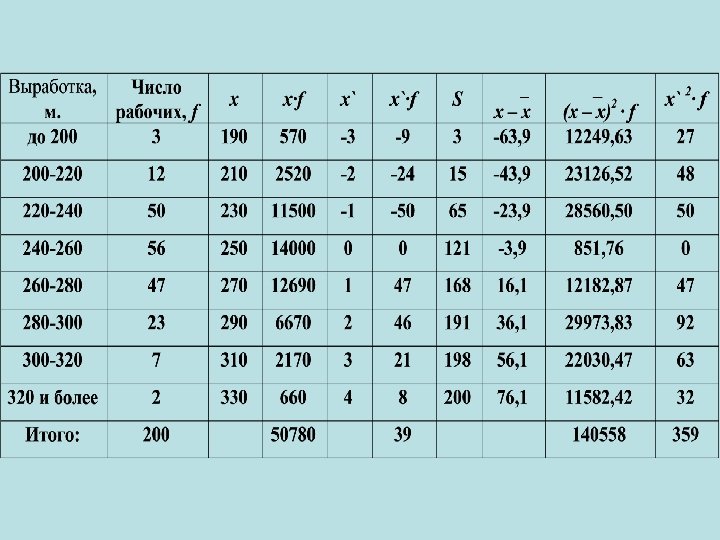
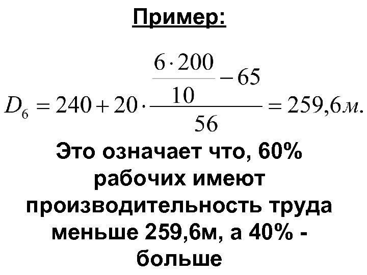
Пример: Это означает что, 60% рабочих имеют производительность труда меньше 259, 6 м, а 40% больше
Применение децилей • Пример - децильный коэффициент дифференциации населения. Население делится на 10 частей по уровню дохода. Берут первые 10% и последние 10%. Считают, что средний доход последней группы не должен быть больше, чем в 10 раз среднего дохода первой группы. В России официально это превышение составляет 1416 раз, неофициально – 20 и более раз
Перцентиль • П делит ранжированную совокупность на 100 равных частей. Формулы аналогичны формулам медианы, квартиля и дециля
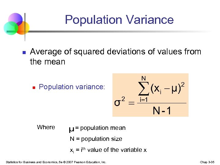
Population Variance n Average of squared deviations of values from the mean n Population variance: Where = population mean N = population size xi = ith value of the variable x Statistics for Business and Economics, 6 e © 2007 Pearson Education, Inc. Chap 3 -35
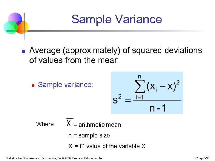
Sample Variance n Average (approximately) of squared deviations of values from the mean n Sample variance: Where = arithmetic mean n = sample size Xi = ith value of the variable X Statistics for Business and Economics, 6 e © 2007 Pearson Education, Inc. Chap 3 -36
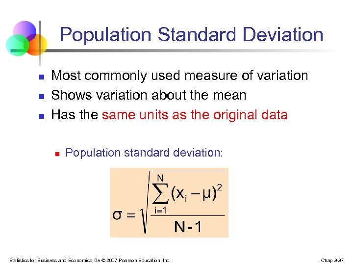
Population Standard Deviation n Most commonly used measure of variation Shows variation about the mean Has the same units as the original data n Population standard deviation: Statistics for Business and Economics, 6 e © 2007 Pearson Education, Inc. Chap 3 -37
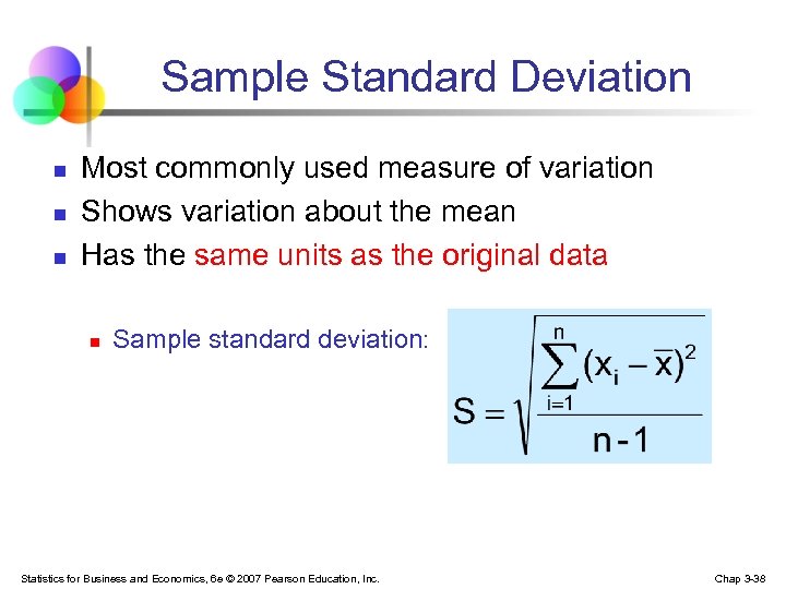
Sample Standard Deviation n Most commonly used measure of variation Shows variation about the mean Has the same units as the original data n Sample standard deviation: Statistics for Business and Economics, 6 e © 2007 Pearson Education, Inc. Chap 3 -38
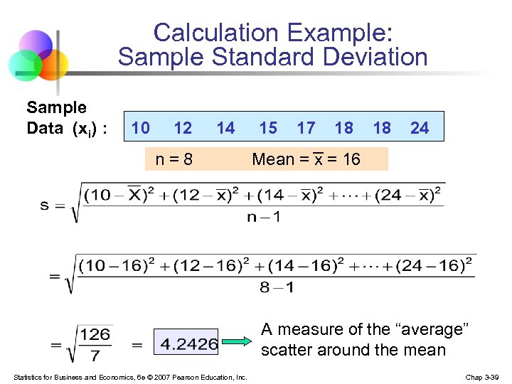
Calculation Example: Sample Standard Deviation Sample Data (xi) : 10 12 14 n=8 15 17 18 18 24 Mean = x = 16 A measure of the “average” scatter around the mean Statistics for Business and Economics, 6 e © 2007 Pearson Education, Inc. Chap 3 -39
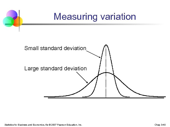
Measuring variation Small standard deviation Large standard deviation Statistics for Business and Economics, 6 e © 2007 Pearson Education, Inc. Chap 3 -40
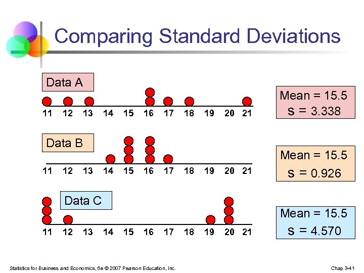
Comparing Standard Deviations Data A 11 12 13 14 15 16 17 18 19 20 21 Mean = 15. 5 s = 3. 338 20 21 Mean = 15. 5 s = 0. 926 20 21 Mean = 15. 5 s = 4. 570 Data B 11 12 13 14 15 16 17 18 19 Data C 11 12 13 14 15 16 17 Statistics for Business and Economics, 6 e © 2007 Pearson Education, Inc. 18 19 Chap 3 -41
Advantages of Variance and Standard Deviation n n Each value in the data set is used in the calculation Values far from the mean are given extra weight (because deviations from the mean are squared) Statistics for Business and Economics, 6 e © 2007 Pearson Education, Inc. Chap 3 -42
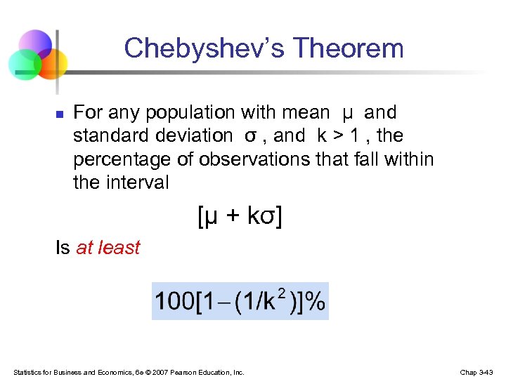
Chebyshev’s Theorem n For any population with mean μ and standard deviation σ , and k > 1 , the percentage of observations that fall within the interval [μ + kσ] Is at least Statistics for Business and Economics, 6 e © 2007 Pearson Education, Inc. Chap 3 -43
Chebyshev’s Theorem (continued) n Regardless of how the data are distributed, at least (1 - 1/k 2) of the values will fall within k standard deviations of the mean (for k > 1) n Examples: At ) = 0% ……. . . k=1 within 1σ) (1 - 1/12 least (μ ± (1 - 1/22) = 75% …. . . . k=2 (μ ± 2σ) (1 - 1/32) = 89% ………. k=3 (μ ± 3σ) Statistics for Business and Economics, 6 e © 2007 Pearson Education, Inc. Chap 3 -44
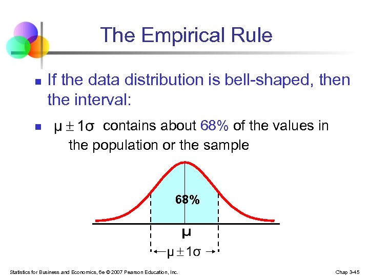
The Empirical Rule n n If the data distribution is bell-shaped, then the interval: contains about 68% of the values in the population or the sample 68% Statistics for Business and Economics, 6 e © 2007 Pearson Education, Inc. Chap 3 -45
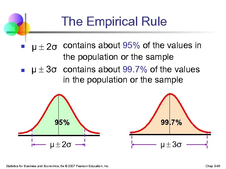
The Empirical Rule n n contains about 95% of the values in the population or the sample contains about 99. 7% of the values in the population or the sample 95% Statistics for Business and Economics, 6 e © 2007 Pearson Education, Inc. 99. 7% Chap 3 -46
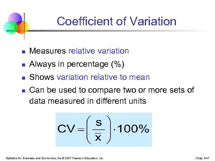
Coefficient of Variation n Measures relative variation n Always in percentage (%) n Shows variation relative to mean n Can be used to compare two or more sets of data measured in different units Statistics for Business and Economics, 6 e © 2007 Pearson Education, Inc. Chap 3 -47
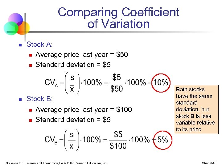
Comparing Coefficient of Variation n n Stock A: n Average price last year = $50 n Standard deviation = $5 Stock B: n n Average price last year = $100 Standard deviation = $5 Statistics for Business and Economics, 6 e © 2007 Pearson Education, Inc. Both stocks have the same standard deviation, but stock B is less variable relative to its price Chap 3 -48

Using Microsoft Excel n Descriptive Statistics can be obtained from Microsoft® Excel n Use menu choice: tools / data analysis / descriptive statistics n Enter details in dialog box Statistics for Business and Economics, 6 e © 2007 Pearson Education, Inc. Chap 3 -49
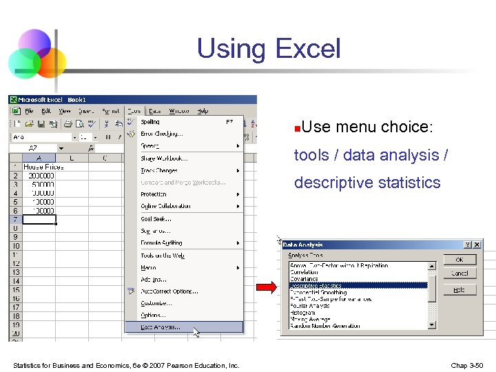
Using Excel n Use menu choice: tools / data analysis / descriptive statistics Statistics for Business and Economics, 6 e © 2007 Pearson Education, Inc. Chap 3 -50
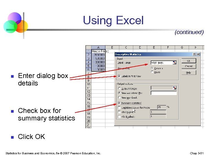
Using Excel (continued) n n n Enter dialog box details Check box for summary statistics Click OK Statistics for Business and Economics, 6 e © 2007 Pearson Education, Inc. Chap 3 -51
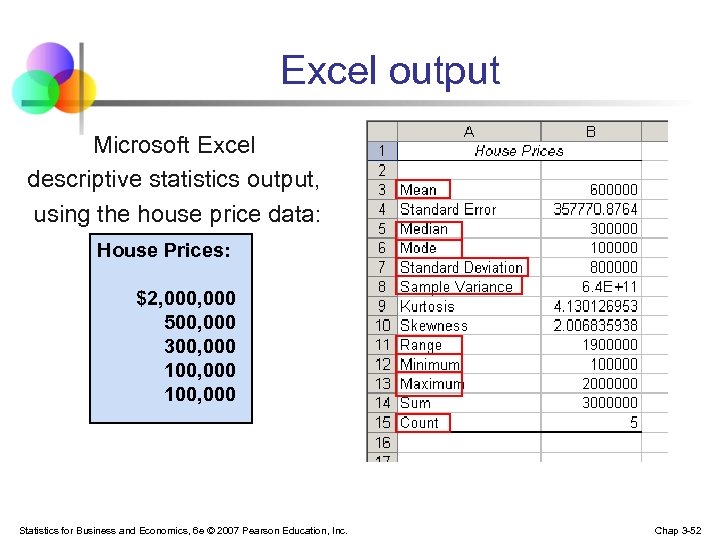
Excel output Microsoft Excel descriptive statistics output, using the house price data: House Prices: $2, 000 500, 000 300, 000 100, 000 Statistics for Business and Economics, 6 e © 2007 Pearson Education, Inc. Chap 3 -52
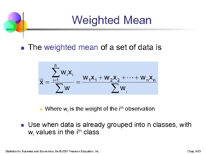
Weighted Mean n The weighted mean of a set of data is n n Where wi is the weight of the ith observation Use when data is already grouped into n classes, with wi values in the ith class Statistics for Business and Economics, 6 e © 2007 Pearson Education, Inc. Chap 3 -53
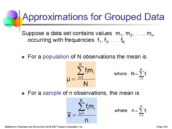
Approximations for Grouped Data Suppose a data set contains values m 1, m 2, . . . , mk, occurring with frequencies f 1, f 2, . . . f. K n For a population of N observations the mean is n For a sample of n observations, the mean is Statistics for Business and Economics, 6 e © 2007 Pearson Education, Inc. Chap 3 -54
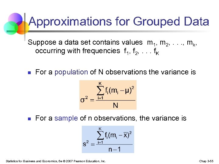
Approximations for Grouped Data Suppose a data set contains values m 1, m 2, . . . , mk, occurring with frequencies f 1, f 2, . . . f. K n For a population of N observations the variance is n For a sample of n observations, the variance is Statistics for Business and Economics, 6 e © 2007 Pearson Education, Inc. Chap 3 -55
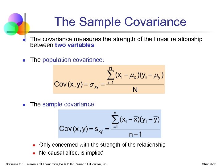
The Sample Covariance n The covariance measures the strength of the linear relationship between two variables n The population covariance: n The sample covariance: n n Only concerned with the strength of the relationship No causal effect is implied Statistics for Business and Economics, 6 e © 2007 Pearson Education, Inc. Chap 3 -56
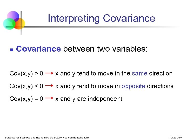
Interpreting Covariance n Covariance between two variables: Cov(x, y) > 0 x and y tend to move in the same direction Cov(x, y) < 0 x and y tend to move in opposite directions Cov(x, y) = 0 x and y are independent Statistics for Business and Economics, 6 e © 2007 Pearson Education, Inc. Chap 3 -57
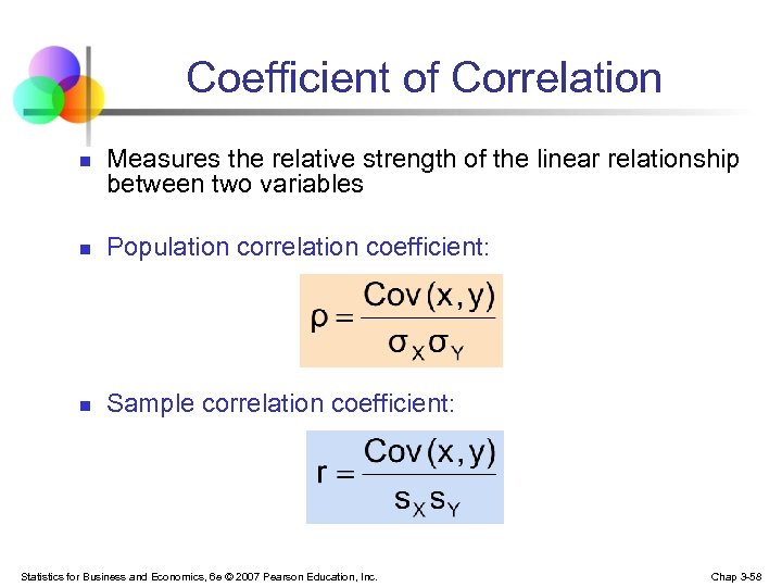
Coefficient of Correlation n Measures the relative strength of the linear relationship between two variables n Population correlation coefficient: n Sample correlation coefficient: Statistics for Business and Economics, 6 e © 2007 Pearson Education, Inc. Chap 3 -58
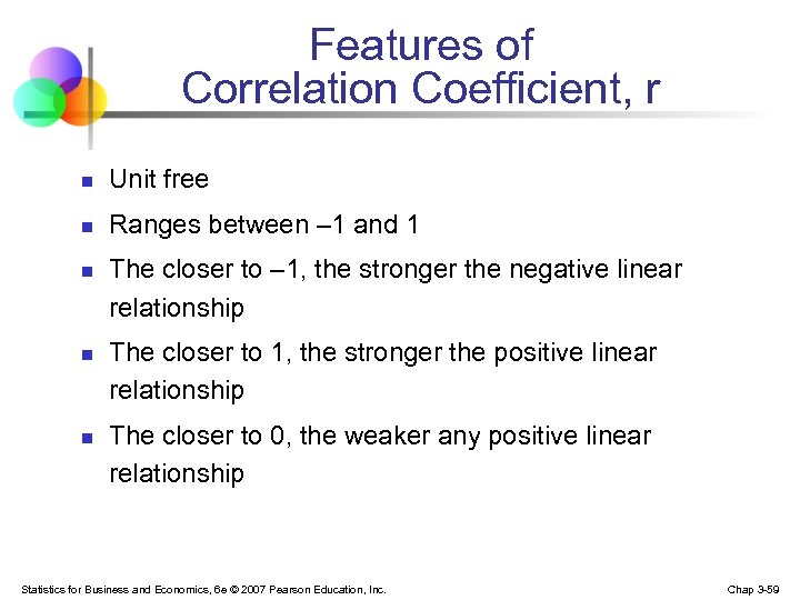
Features of Correlation Coefficient, r n Unit free n Ranges between – 1 and 1 n n n The closer to – 1, the stronger the negative linear relationship The closer to 1, the stronger the positive linear relationship The closer to 0, the weaker any positive linear relationship Statistics for Business and Economics, 6 e © 2007 Pearson Education, Inc. Chap 3 -59
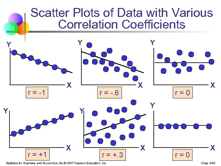
Scatter Plots of Data with Various Correlation Coefficients Y Y r = -1 X Y Y r = -. 6 X Y Y r = +1 X r=0 X r = +. 3 Statistics for Business and Economics, 6 e © 2007 Pearson Education, Inc. X r=0 X Chap 3 -60
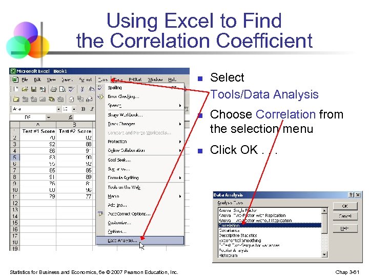
Using Excel to Find the Correlation Coefficient n n n Statistics for Business and Economics, 6 e © 2007 Pearson Education, Inc. Select Tools/Data Analysis Choose Correlation from the selection menu Click OK. . . Chap 3 -61
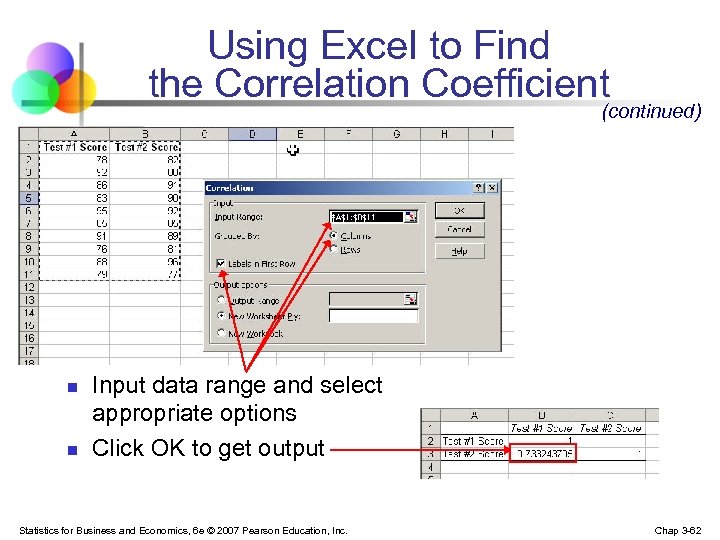
Using Excel to Find the Correlation Coefficient (continued) n n Input data range and select appropriate options Click OK to get output Statistics for Business and Economics, 6 e © 2007 Pearson Education, Inc. Chap 3 -62
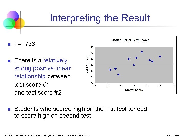
Interpreting the Result n n n r =. 733 There is a relatively strong positive linear relationship between test score #1 and test score #2 Students who scored high on the first tended to score high on second test Statistics for Business and Economics, 6 e © 2007 Pearson Education, Inc. Chap 3 -63
Obtaining Linear Relationships n An equation can be fit to show the best linear relationship between two variables: Y = β 0 + β 1 X Where Y is the dependent variable and X is the independent variable Statistics for Business and Economics, 6 e © 2007 Pearson Education, Inc. Chap 3 -64
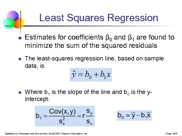
Least Squares Regression n Estimates for coefficients β 0 and β 1 are found to minimize the sum of the squared residuals The least-squares regression line, based on sample data, is Where b 1 is the slope of the line and b 0 is the yintercept: Statistics for Business and Economics, 6 e © 2007 Pearson Education, Inc. Chap 3 -65
Chapter Summary n Described measures of central tendency n n Illustrated the shape of the distribution n Symmetric, skewed Described measures of variation n n Mean, median, mode Range, interquartile range, variance and standard deviation, coefficient of variation Discussed measures of grouped data Calculated measures of relationships between variables n covariance and correlation coefficient Statistics for Business and Economics, 6 e © 2007 Pearson Education, Inc. Chap 3 -66
c9e367941f6a9d37e01dbaf1ef91187d.ppt