Variance estimation for Generalized Entropy and Atkinson inequality

Variance estimation for Generalized Entropy and Atkinson inequality indices: the complex survey data case Martin Biewen (Goethe University Frankfurt) Stephen Jenkins (University of Essex) Presentation at 4 th German Stata User Group Meeting, Mannheim, 31 March 2006

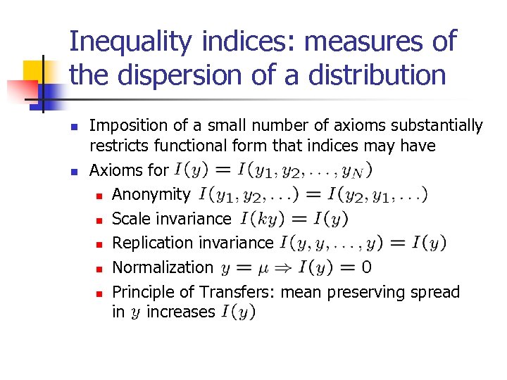Inequality indices: measures of the dispersion of a distribution n n Imposition of a small number of axioms substantially restricts functional form that indices may have Axioms for n Anonymity n Scale invariance n Replication invariance n Normalization n Principle of Transfers: mean preserving spread in increases

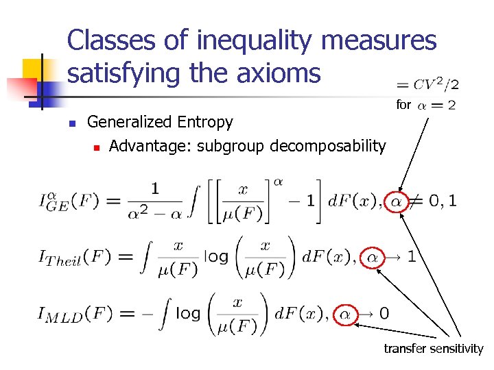Classes of inequality measures satisfying the axioms for n Generalized Entropy n Advantage: subgroup decomposability transfer sensitivity

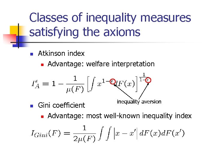Classes of inequality measures satisfying the axioms n n Atkinson index n Advantage: welfare interpretation inequality aversion Gini coefficient n Advantage: most well-known inequality index

Estimation of inequality indices n n These indices are routinely calculated by many analysts … n The most commonly-used programs among Stata users are ineqdeco and inequal 7 (available using ssc) But only rarely do analysts report estimates of the associated sampling variances (or SEs) of the estimates!

Estimation of inequality indices n n Analytical derivations to date have omitted some important situations (and indices) n Most derivations assume i. i. d. observations (cf. survey clustering or other sample dependencies!), and don‘t consider probability weighting (cf. stratification!) n The methods that do exist are not ‘well known’ Lack of available software n But cf. geivars (Cowell (1989), linearization methods; i. i. d. assumptions) and ineqerr (bootstrap), both available using ssc

What we provide n n n Estimates of indices and associated sampling variances for all members of the GE and Atkinson classes, while also … Accounting for clustering and stratification, and for the i. i. d. case Analytical results (see our paper) and new Stata programs (version 8. 2): svygei and svyatk Based on Taylor-series linearization methods combined with a result from Woodruff (JASA, 1971). Results don‘t apply to Gini coefficient.

Overview of analytical derivation n n Write estimator of each index as a function of population totals (involves sums over clusters, weights etc. ) (Taylor-series approximation) Variance of each estimator can be approximated by variance of 1 st order ‘residual’ As is, each expression is not easily calculated … But (Woodruff): reversing order of summation in ‘residual’ → estimation is equivalent to derivation of a sampling variance of a total estimator for which one can apply standard svy methods

The programs: svygei and svyatk svygei varname [if exp] [in range] [, alpha(#) subpop(varname) level(#) Calculations for (use alpha(#) option to chose one other than ) svyatk varname [if exp] [in range] [, epsilon(#) subpop(varname) level(#) Calculations for (use epsilon(#) option to chose one other than n n ) Where, of course, the data have first been svyset. How data are organised, and described using svyset is of crucial importance …

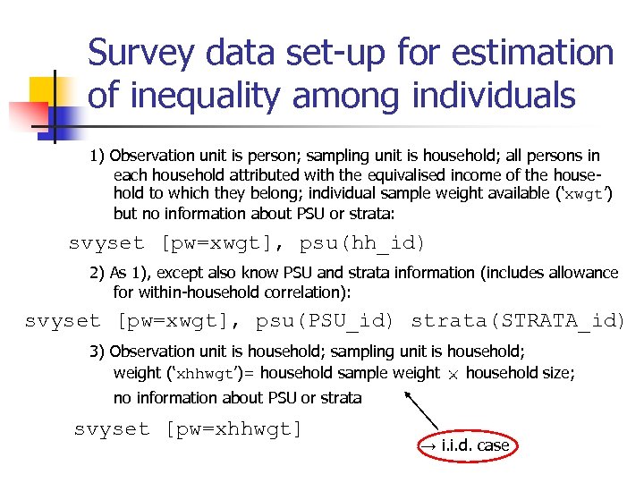Survey data set-up for estimation of inequality among individuals 1) Observation unit is person; sampling unit is household; all persons in each household attributed with the equivalised income of the household to which they belong; individual sample weight available (‘xwgt’) but no information about PSU or strata: svyset [pw=xwgt], psu(hh_id) 2) As 1), except also know PSU and strata information (includes allowance for within-household correlation): svyset [pw=xwgt], psu(PSU_id) strata(STRATA_id) 3) Observation unit is household; sampling unit is household; weight (‘xhhwgt’)= household sample weight household size; no information about PSU or strata svyset [pw=xhhwgt] → i. i. d. case

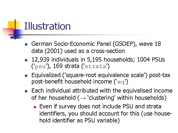Illustration n n German Socio-Economic Panel (GSOEP), wave 18 data (2001) used as a cross-section 12, 939 individuals in 5, 195 households; 1004 PSUs (‘psu’), 169 strata (‘strata’) Equivalized (‘square-root equivalence scale’) post-tax post-benefit household income (‘eq’) Each individual attributed with the equivalised income of her household (→ ‘clustering’ within households) n Even if survey does not include PSU and strata identifiers, you should account for this (use household identifier as PSU variable)

Generalized Entropy indices. ssc install svygei_svyatk. version 8. 2. svyset [pweight=xwgt], psu(psu) strata(strata). svygei eq Complex survey estimates of Generalized Entropy inequality indices pweight: xwgt Strata: strata PSU: psu Number of obs = 12939 Number of strata = 169 Number of PSUs = 1004 Population size = 31487411 -------------------------------------Index | Estimate Std. Err. z P>|z| [95% Conf. Interval] -----+--------------------------------GE(-1) |. 1179647. 00614786 19. 19 0. 000. 1059151. 1300143 MLD |. 1020797. 00495919 20. 58 0. 000. 0923599. 1117996 Theil |. 1027892. 0058706 17. 51 0. 000. 091283. 1142954 GE(2) |. 1201693. 00962991 12. 48 0. 000. 101295. 1390436 GE(3) |. 1713159. 02301064 7. 45 0. 000. 1262159. 2164159 --------------------------------------

Atkinson indices. svyset [pweight=xwgt], psu(psu) strata(strata). svyatk eq Complex survey estimates of Atkinson inequality indices pweight: xwgt Strata: strata PSU: psu Number of obs = 12939 Number of strata = 169 Number of PSUs = 1004 Population size = 31487411 -------------------------------------Index | Estimate Std. Err. z P>|z| [95% Conf. Interval] -----+--------------------------------A(0. 5) |. 0496963. 0025263 19. 67 0. 000. 0447448. 0546477 A(1) |. 0970424. 00447794 21. 67 0. 000. 0882658. 105819 A(1. 5) |. 1434968. 00616915 23. 26 0. 000. 1314055. 1555881 A(2) |. 1908923. 00804946 23. 71 0. 000. 1751157. 206669 A(2. 5) |. 2432834. 01237288 19. 66 0. 000. 219033. 2675338 --------------------------------------

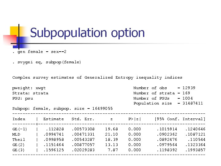Subpopulation option. gen female = sex==2. svygei eq, subpop(female) Complex survey estimates of Generalized Entropy inequality indices pweight: xwgt Strata: strata PSU: psu Number of obs Number of strata Number of PSUs Population size = = 12939 169 1004 31487411 Subpop: female, subpop. size = 16499055 -------------------------------------Index | Estimate Std. Err. z P>|z| [95% Conf. Interval] -----+--------------------------------GE(-1) |. 112828. 00573308 19. 68 0. 000. 1015914. 1240646 MLD |. 0994741. 00471331 21. 10 0. 000. 0902362. 1087121 Theil |. 0998958. 00543287 18. 39 0. 000. 0892476. 110544 GE(2) |. 1151464. 00877057 13. 13 0. 000. 0979564. 1323364 GE(3) |. 1596125. 02029283 7. 87 0. 000. 1198392. 1993857 --------------------------------------

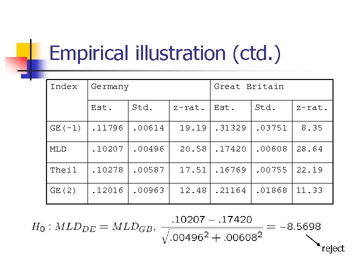
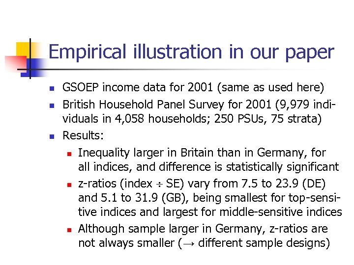Empirical illustration in our paper n n n GSOEP income data for 2001 (same as used here) British Household Panel Survey for 2001 (9, 979 individuals in 4, 058 households; 250 PSUs, 75 strata) Results: n Inequality larger in Britain than in Germany, for all indices, and difference is statistically significant n z-ratios (index SE) vary from 7. 5 to 23. 9 (DE) and 5. 1 to 31. 9 (GB), being smallest for top-sensitive indices and largest for middle-sensitive indices n Although sample larger in Germany, z-ratios are not always smaller (→ different sample designs)

Empirical illustration (ctd. ) Index Germany Est. Great Britain Std. z-rat. Est. Std. z-rat. GE(-1). 11796. 00614 19. 31329. 03751 8. 35 MLD . 10207. 00496 20. 58. 17420. 00608 28. 64 Theil . 10278. 00587 17. 51. 16769. 00755 22. 19 GE(2) . 12016. 00963 12. 48. 21164. 01868 11. 33 reject

Empirical illustration (ctd. ) n Effects of different assumptions about survey design on sampling variance estimates? n For each index, the estimated standard error is larger if one accounts for survey clustering and stratification (unsurprising), but … n Results suggest that accounting for survey design features per se have little (additional) effect on variance estimates as long as the replication of incomes within multi-person households is accounted for

Conclusions n Researchers now have the means to estimate sampling variances for most of the inequality indices in common use, accomodating a range of potential assumptions about design effects Topics for future research: n GE indices are additively decomposable by population subgroup (→ ineqdeco): extend results here to the components of decompositions n Extend results to Gini coefficient and other measures based on order-statistics (Lorenz curves etc. )

Selected references n Biewen, M. and Jenkins S. P. (2006): Estimation of Generalized Entropy and Atkinson indices from complex survey data, forthcoming in: Oxford Bulletin of Economics and Statistics n n Cowell, F. A. (2000): Measurement of inequality, in A. B. Atkinson and F. Bourguignon (eds), Handbook of Income Distribution, Vol. 1, Elsevier, Amsterdam Woodruff, R. S. (1971): A simple method for approximating the variance of a complicated estimate, Journal of the American Statistical Association, 66, 411 -4