Variability and Uncertainty Introduction Stochastic Programming Robust Programming

Variability and Uncertainty Introduction Stochastic Programming Robust Programming Multiparametric Programming Dynamic Programming Plantilla -10

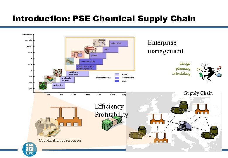
Introduction: PSE Chemical Supply Chain Enterprise management design planning scheduling Supply Chain Efficiency Profitability Coordination of resources 2

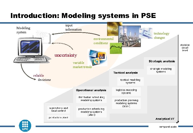
Introduction: Modeling systems in PSE input information Modeling system environmental conditions technology changes uncertainty variable market trends reliable decisions 3

Introduction: Uncertainty n The model will include a series of uncertain parameters u There is not a unique solution… u There is not an optimal solution… n In spite of this, a decision should be made u (before the uncertainty is revealed) n Solution based on average values (or nominal values) does not need to be the best u It could be even unfeasible n Decision making implies a risk u Typically, there will be a trade-off among expected efficiency and assumed risk n Prediction is very difficult… specially about the future Niels Bohr Plantilla -40

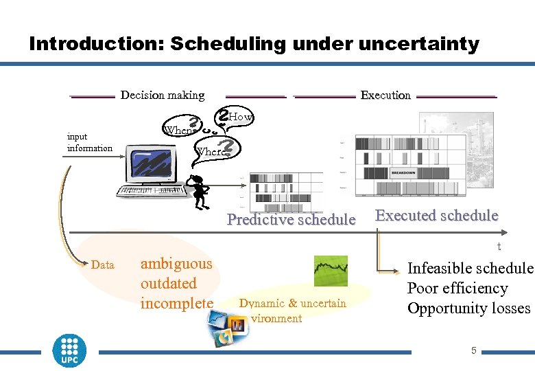
Introduction: Scheduling under uncertainty Decision making input information Execution How When Where Predictive schedule Executed schedule t Data ambiguous outdated incomplete Dynamic & uncertain environment Infeasible schedule Poor efficiency Opportunity losses 5

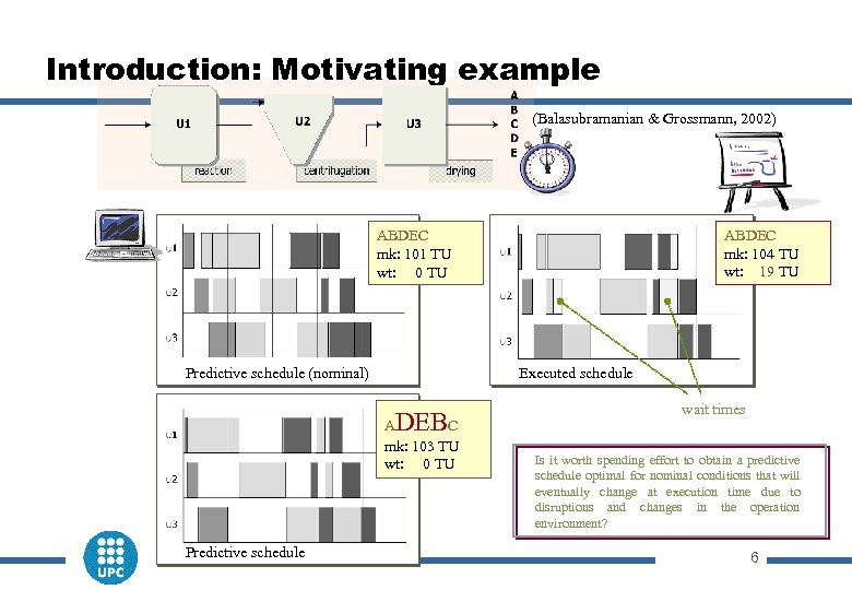
Introduction: Motivating example (Balasubramanian & Grossmann, 2002) ABDEC mk: 104 TU wt: 19 TU ABDEC mk: 101 TU wt: 0 TU Predictive schedule (nominal) Executed schedule DEB A C mk: 103 TU wt: 0 TU Predictive schedule wait times Is it worth spending effort to obtain a predictive schedule optimal for nominal conditions that will eventually change at execution time due to disruptions and changes in the operation environment? 6

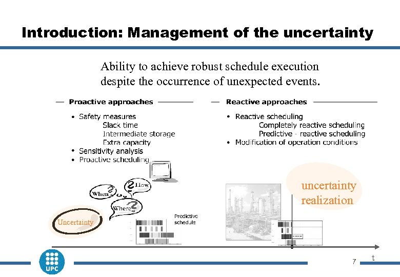
Introduction: Management of the uncertainty Ability to achieve robust schedule execution despite the occurrence of unexpected events. uncertainty realization Uncertainty 7 t

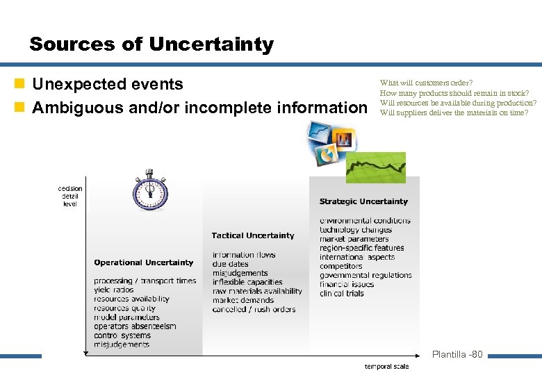
Sources of Uncertainty n Unexpected events n Ambiguous and/or incomplete information What will customers order? How many products should remain in stock? Will resources be available during production? Will suppliers deliver the materials on time? Plantilla -80

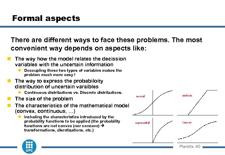
Formal aspects There are different ways to face these problems. The most convenient way depends on aspects like: n The way how the model relates the decission variables with the uncertain information u Decoupling these two types of variables makes the problem much more easy ! n The way to express the probabiloity distribution of uncertain varaibles u Continuous distributions vs. Discrete distributions. n The size of the problem n The characteristics of the mathematical model (convex, continuous, …) u Including the characteristics introduced by the probability functions to be applied (the probability functions are not convex (nor concave) transformations, disretizations, etc. ) Plantilla -90

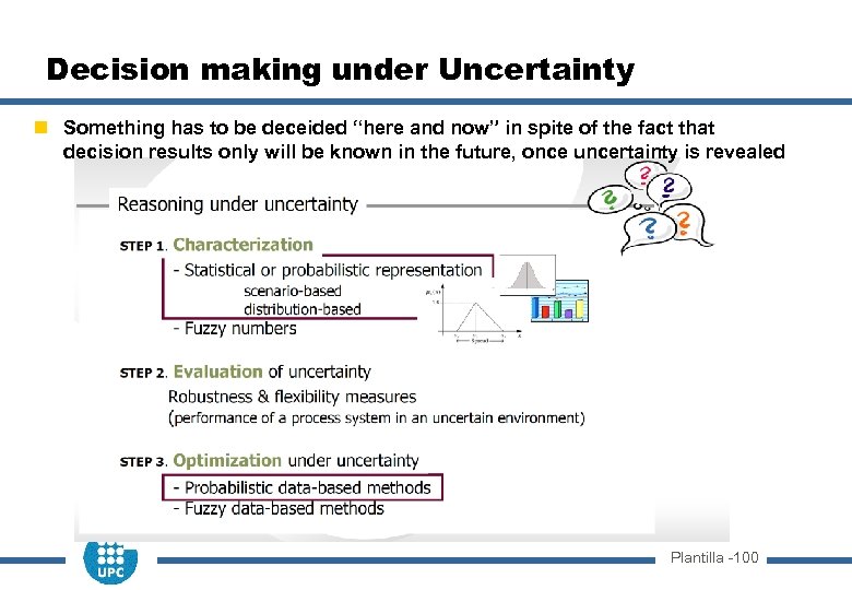
Decision making under Uncertainty n Something has to be deceided “here and now” in spite of the fact that decision results only will be known in the future, once uncertainty is revealed Plantilla -100

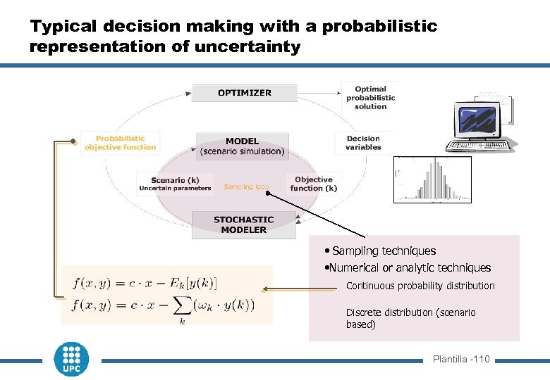
Typical decision making with a probabilistic representation of uncertainty • Sampling techniques • Numerical or analytic techniques Continuous probability distribution Discrete distribution (scenario based) Plantilla -110

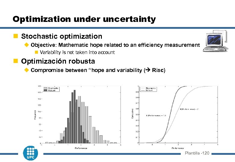
Optimization under uncertainty n Stochastic optimization u Objective: Mathematic hope related to an efficiency measurement n Variability is not taken into account n Optimización robusta u Compromise between “hope and variability ( Risc) Plantilla -120

1. - Stochastic Programming n Combines the power of mathematical programming with statistical advanced techniques: u Convexity analysis, development of dual problems, … problem decomposition u Constraints management n The solution procedures are driven by the formalization of the probability model. u For example: When the number of scenarios to be contemplated is discrete Deterministic equivalent problem (the size of the problem will be basically a function of the number of scenarios to be considered) Plantilla -130

General Methods of stochastic programming n Multi-step methods(multistage stochastic programming): u Penalization (“recourse problems”): The potential losses caused by uncertainty are “a posteriori” compensated solving another optimization problem. u This second problem depend on the decisions already made (“first step”) and on the uncertainty finally revealed. n The variable associated to this new optimization is the “resource” required to compensate the uncertainty effects. u During the first step decision making, the eventual (uncertain) values of the second stage variables are explicitly considered u Limitations: n Not applicable if the decisions (and states) affect the probability distribution n The costs associated to the “resource decisions” should be known in advance. n Chance-constrained programming: some constraints do not need to be maintained in a limited number of cases. Plantilla -140

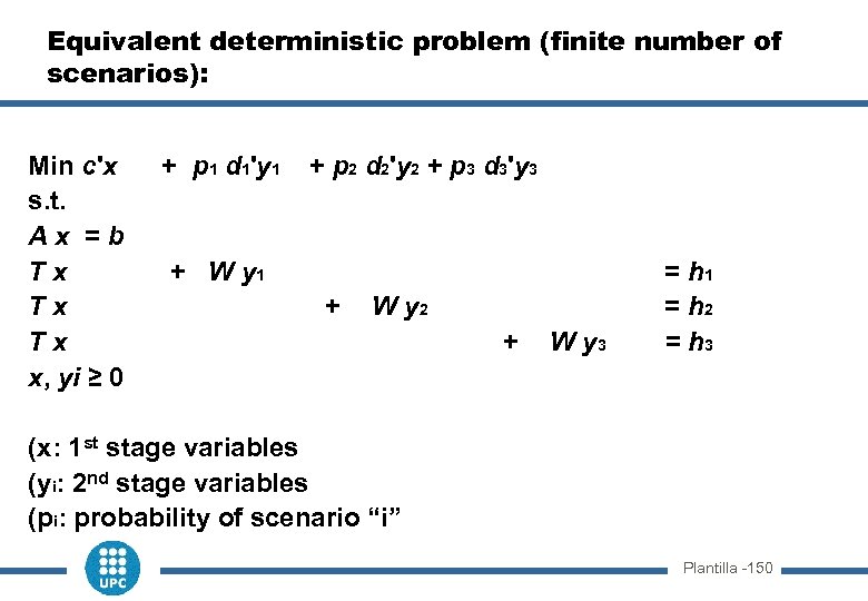
Equivalent deterministic problem (finite number of scenarios): Min c'x + p 1 d 1'y 1 + p 2 d 2'y 2 + p 3 d 3'y 3 s. t. A x = b T x + W y 1 = h 1 T x + W y 2 = h 2 T x + W y 3 = h 3 x, yi ≥ 0 (x: 1 st stage variables (yi: 2 nd stage variables (pi: probability of scenario “i” Plantilla -150

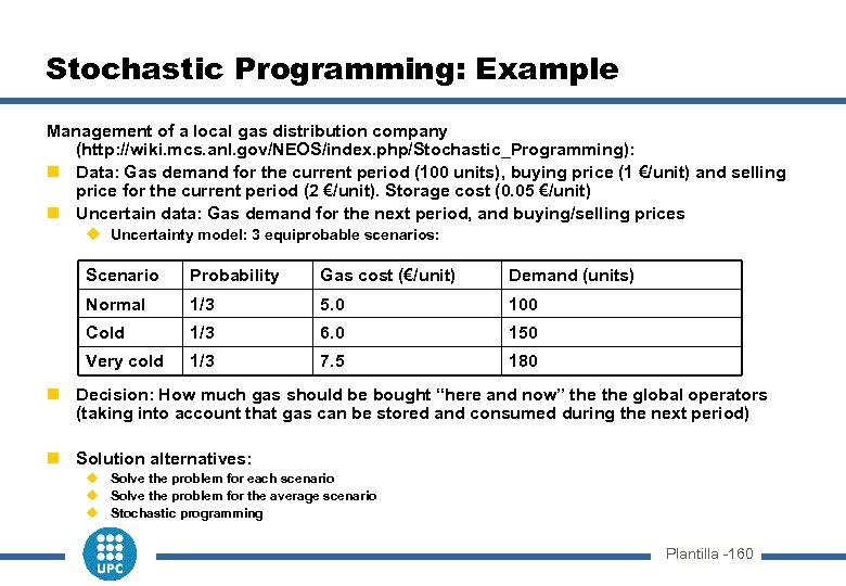
Stochastic Programming: Example Management of a local gas distribution company (http: //wiki. mcs. anl. gov/NEOS/index. php/Stochastic_Programming): n Data: Gas demand for the current period (100 units), buying price (1 €/unit) and selling price for the current period (2 €/unit). Storage cost (0. 05 €/unit) n Uncertain data: Gas demand for the next period, and buying/selling prices u Uncertainty model: 3 equiprobable scenarios: Scenario Probability Gas cost (€/unit) Demand (units) Normal 1/3 5. 0 100 Cold 1/3 6. 0 150 Very cold 1/3 7. 5 180 n Decision: How much gas should be bought “here and now” the global operators (taking into account that gas can be stored and consumed during the next period) n Solution alternatives: u Solve the problem for each scenario u Solve the problem for the average scenario u Stochastic programming Plantilla -160

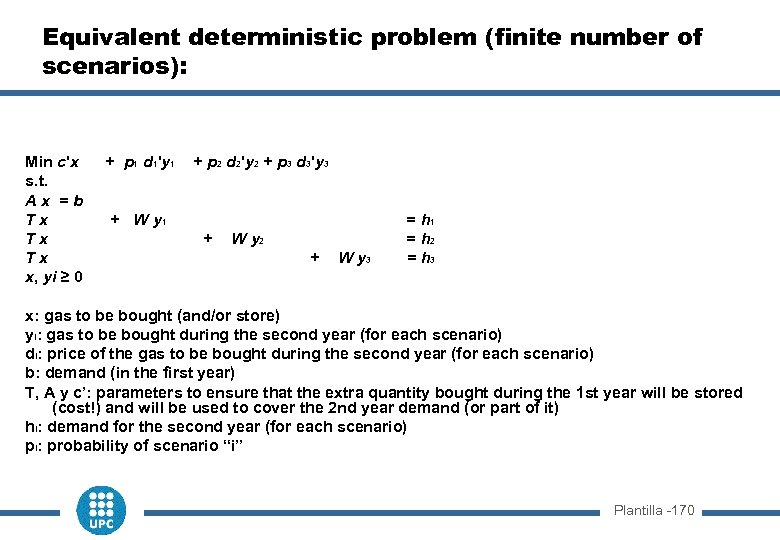
Equivalent deterministic problem (finite number of scenarios): Min c'x + p 1 d 1'y 1 + p 2 d 2'y 2 + p 3 d 3'y 3 s. t. A x = b T x + W y 1 = h 1 T x + W y 2 = h 2 T x + W y 3 = h 3 x, yi ≥ 0 x: gas to be bought (and/or store) yi: gas to be bought during the second year (for each scenario) di: price of the gas to be bought during the second year (for each scenario) b: demand (in the first year) T, A y c’: parameters to ensure that the extra quantity bought during the 1 st year will be stored (cost!) and will be used to cover the 2 nd year demand (or part of it) hi: demand for the second year (for each scenario) pi: probability of scenario “i” Plantilla -170

Mathematical formulation One unique scenario Minimize (sum Price[t] * Buy[t]) + (sum Store[t] * Storage. Cost) subject to: Buy[t] + Use_stored[t] >= Demand[t], t in (1, 2) Store[t] = Store[t-1] + Buy[t] - Demand[t], t in (1, 2) Use_stored[t] <= Store[t-1], t in (1, 2) “n” scenarios Minimize (Price[1][1] * Buy[1][1] + sum Store[1][1] * Storage. Cost) + + sum Scen Prob[Scen] * (Price[2][Scen] * Buy[2][Scen] + Store[2][Scen] * Storage. Cost) First-period constraints Buy[1][1] + Use_stored[1][1] >= Demand[1][1] Store[1] = Store[0] + Buy[1] - Demand[1] Use_stored[1] <= Store[0] Second-period constraints Buy[2][Scen] + Use_stored[2][Scen] >= Demand[2][Scen] Store[2][Scen] = Store[1][1] + Buy[2][Scen] - Demand[1][Scen] Use_stored[2][Scen] <= Store[1][1] Plantilla -180

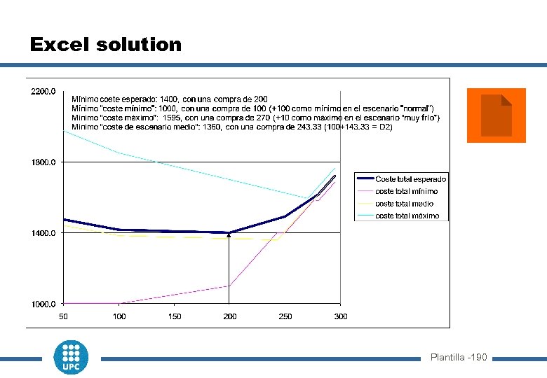
Excel solution Plantilla -190

“Chance constrained” programming Equivalent to stochastic programming, including a new constraint to limit the probability of not matching a certain constraint to a certain maximum value. Examples: Same problem u including a constraint to limit the probability of having to buy more than 30 units in the second period u. Accepting solutions no covering the 10% of the second year demand in a 5% of the eventual situations n Helps to assess the “parameters” probability distribution Plantilla -200

2. - Robust programming The model includes a series of “i” unknow parameters (si); although their value is unknown, they should be among a specific set of specific values (Si) n Optimization = To look for the best solution which meets all constraints ( feasibility) for any parameters value combination u Worst Case Analysis for any eventual decision u (The set of scenarions is, actually, i irrelevant “S”: Set of “s” = uncertain parameters (preferably: continuous and convex) Variation: To look for the best solution which meets all constraints ( feasibility) which a probability less than “alfa” to get a result worst than “zmin” (“downside risk”) Plantilla -210

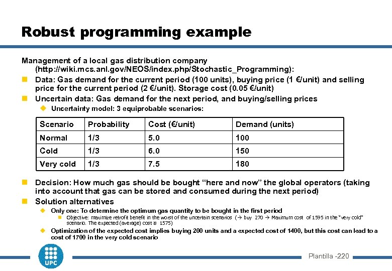
Robust programming example Management of a local gas distribution company (http: //wiki. mcs. anl. gov/NEOS/index. php/Stochastic_Programming): n Data: Gas demand for the current period (100 units), buying price (1 €/unit) and selling price for the current period (2 €/unit). Storage cost (0. 05 €/unit) n Uncertain data: Gas demand for the next period, and buying/selling prices u Uncertainty model: 3 equiprobable scenarios: Scenario Probability Cost (€/unit) Demand (units) Normal 1/3 5. 0 100 Cold 1/3 6. 0 150 Very cold 1/3 7. 5 180 n Decision: How much gas should be bought “here and now” the global operators (taking into account that gas can be stored and consumed during the next period) n Solution alternatives u Only one: To determine the optimum gas quantity to be bought in the first period n Objective: maximize retrofit benefit in the worst of the uncertain scenarios ( buy 270 Maximum cost of 1595 in the “very cold” scenario. The expected (average) cost is 1575) u Optimization of the expected cost implies buying 200 units and a expected cost of 1400, but this cost can lead to a cost of 1700 in the very cold scenario Plantilla -220

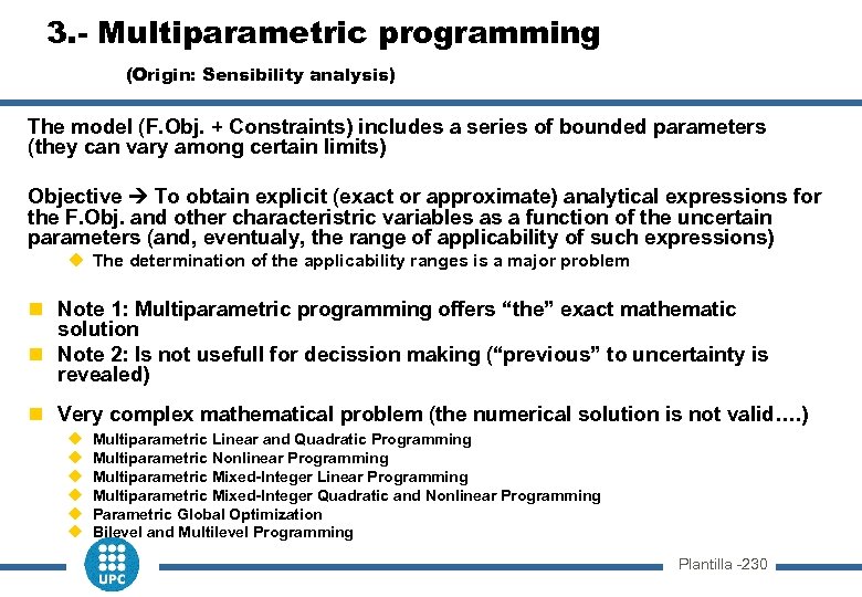
3. - Multiparametric programming (Origin: Sensibility analysis) The model (F. Obj. + Constraints) includes a series of bounded parameters (they can vary among certain limits) Objective To obtain explicit (exact or approximate) analytical expressions for the F. Obj. and other characteristric variables as a function of the uncertain parameters (and, eventualy, the range of applicability of such expressions) u The determination of the applicability ranges is a major problem n Note 1: Multiparametric programming offers “the” exact mathematic solution n Note 2: Is not usefull for decission making (“previous” to uncertainty is revealed) n Very complex mathematical problem (the numerical solution is not valid…. ) u u u Multiparametric Linear and Quadratic Programming Multiparametric Nonlinear Programming Multiparametric Mixed-Integer Linear Programming Multiparametric Mixed-Integer Quadratic and Nonlinear Programming Parametric Global Optimization Bilevel and Multilevel Programming Plantilla -230

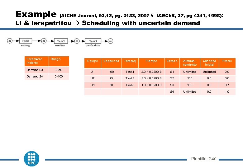
Example (AICHE Journal, 53, 12, pg. 3183, 2007 // I&ECh. R, 37, pg 4341, 1998): Li & Ierapetritou Scheduling with uncertain demand Parámetro Incierto Rango Demand S 3 0 -50 Demand S 4 0 -100 Equipo Capacidad Tarea(s) Tiempo Estado Almace namiento Cantidad Inicial Precio U 1 100 Task 1 3. 0 + 0. 0300 B S 1 Unlimited 0. 0 U 2 75 Task 2 2. 0 + 0. 0266 B S 2 100 0. 0 U 3 50 Task 3 1. 0 + 0. 0200 B S 3 100 0. 7 S 4 Unlimited 0. 0 1. 0 Plantilla -240

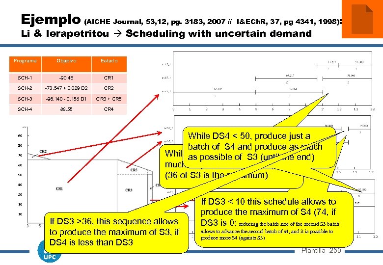
Ejemplo (AICHE Journal, 53, 12, pg. 3183, 2007 // I&ECh. R, 37, pg 4341, 1998): Li & Ierapetritou Scheduling with uncertain demand Programa Objetivo Estado SCH-1 -90. 46 CR 1 SCH-2 -73. 547 + 0. 029 D 2 CR 2 SCH-3 -96. 140 - 0. 158 D 1 CR 3 + CR 5 SCH-4 88. 55 CR 4 90 80 70 60 50 While DS 4 < 50, produce just a batch of S 4 and produce as much While as possibleproduce as the end) DS 3 < 36, of S 3 (until much as possible of S 4 (65) (36 of S 3 is the maximum) 40 30 20 10 If DS 3 >36, this sequence allows to produce the maximum of S 3, if DS 4 is less than DS 3 If DS 3 < 10 this schedule allows to produce the maximum of S 4 (74, if DS 3 is 0: reducing the batch size of the second S 3 batch allows to advance the second batch of s 4, and it is possible to produce more S 4 (againts S 3) Plantilla -250

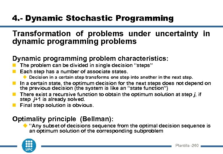
4. - Dynamic Stochastic Programming Transformation of problems under uncertainty in dynamic programming problems Dynamic programming problem characteristics: n The problem can be divided in single decision “steps” n Each step has a number of associate states. u Decision in a certain step transforms one step into another in the next step. n In a certain state, the optimum decision for the next steps does not depend on the previous decision (the system is like an “state function”) n There exist a recursive function to obtain the optimum solution at step j, if step j+1 is already solved. n Final step solution is obvious. Optimality principle (Bellman): u “Any subset of decisions sequence from the optimal decision sequence is an optimum solution of the corresponding subproblem Plantilla -260

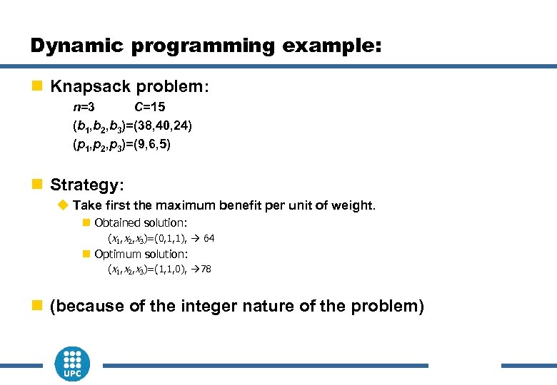
Dynamic programming example: n Knapsack problem: n=3 C=15 (b 1, b 2, b 3)=(38, 40, 24) (p 1, p 2, p 3)=(9, 6, 5) n Strategy: u Take first the maximum benefit per unit of weight. n Obtained solution: (x 1, x 2, x 3)=(0, 1, 1), 64 n Optimum solution: (x 1, x 2, x 3)=(1, 1, 0), 78 n (because of the integer nature of the problem)

Dynamic programming: Introduction R. Bellman: Dynamic Programming, Princeton University Press, 1957. u Se emplea típicamente para resolver problemas de optimización. u Permite resolver problemas mediante una secuencia de decisiones. Como el esquema voraz u A diferencia del esquema voraz, se producen varias secuencias de decisiones (d 1, d 2, …, dn) y solo al final se sabe cuál es la mejor de ellas. n Si hay «o» opciones posibles para cada una de las decisiones, una técnica de fuerza bruta exploraría un total de on secuencias posibles de decisiones (explosión combinatoria). n La programación dinámica evita explorar todas las secuencias posibles por medio de la resolución de subproblemas de tamaño creciente y almacenamiento en una tabla de las soluciones óptimas de esos subproblemas para facilitar la solución de los problemas más grandes.

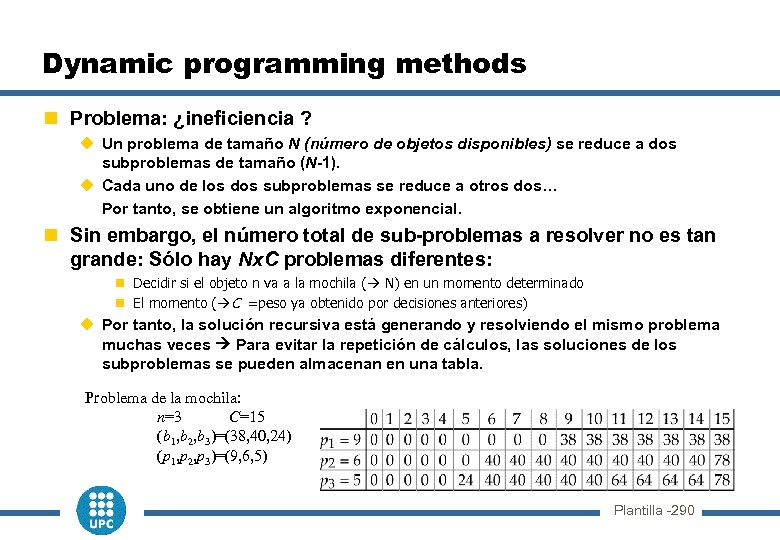
Dynamic programming methods n Problema: ¿ineficiencia ? u Un problema de tamaño N (número de objetos disponibles) se reduce a dos subproblemas de tamaño (N-1). u Cada uno de los dos subproblemas se reduce a otros dos… Por tanto, se obtiene un algoritmo exponencial. n Sin embargo, el número total de sub-problemas a resolver no es tan grande: Sólo hay Nx. C problemas diferentes: n Decidir si el objeto n va a la mochila ( N) en un momento determinado n El momento ( C =peso ya obtenido por decisiones anteriores) u Por tanto, la solución recursiva está generando y resolviendo el mismo problema muchas veces Para evitar la repetición de cálculos, las soluciones de los subproblemas se pueden almacenan en una tabla. Problema de la mochila: n=3 C=15 (b 1, b 2, b 3)=(38, 40, 24) (p 1, p 2, p 3)=(9, 6, 5) Plantilla -290

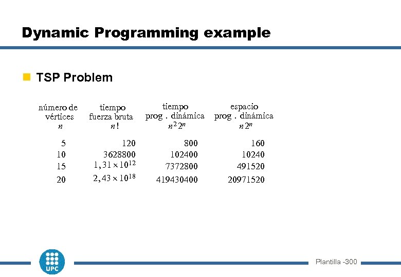
Dynamic Programming example n TSP Problem número de vértices n 5 10 15 20 tiempo fuerza bruta n! 120 3628800 1, 31 1012 2, 43 1018 tiempo prog. dinámica n 2 2 n espacio prog. dinámica n 2 n 800 102400 7372800 419430400 160 10240 491520 20971520 Plantilla -300

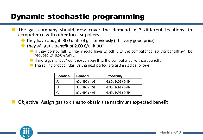
Dynamic stochastic programming n The gas company should now cover the demand in 3 different locations, in competence with other local suppliers. u They have bought 300 units of gas previously (at a very good price) u They will get a benefit of 2. 00 €/unit BUT n If they do not sell it, they should have to sell it to the competence, so the benefit will be reduced to 0. 50 €/unit. n If more gas is required, they can buy it to the competence, without benefit. n The selling probabilities for the next period are estimated as follows: Location Demand Probability A 50 / 100 / 150 0. 60 / 0. 00 / 0. 40 B 50 / 100 / 150 0. 50 / 0. 10 / 0. 40 C 50 / 100 / 150 0. 40 / 0. 30 n Objective: Assign gas to cities to obtain the maximum expected benefit Plantilla -310

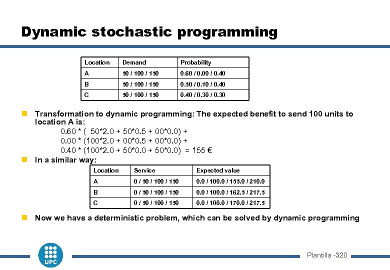
Dynamic stochastic programming Location Demand Probability A 50 / 100 / 150 0. 60 / 0. 00 / 0. 40 B 50 / 100 / 150 0. 50 / 0. 10 / 0. 40 C 50 / 100 / 150 0. 40 / 0. 30 n Transformation to dynamic programming: The expected benefit to send 100 units to location A is: 0. 60 * ( 50*2. 0 + 50*0. 5 + 00*0. 0) + 0. 00 * (100*2. 0 + 00*0. 5 + 00*0. 0) + 0. 40 * (100*2. 0 + 50*0. 0) = 155 € n In a similar way: Location Service Expected value A 0 / 50 / 100 / 150 0. 0 / 100. 0 / 155. 0 / 210. 0 B 0 / 50 / 100 / 150 0. 0 / 100. 0 / 162. 5 / 217. 5 C 0 / 50 / 100 / 150 0. 0 / 100. 0 / 170. 0 / 217. 5 n Now we have a deterministic problem, which can be solved by dynamic programming Plantilla -320

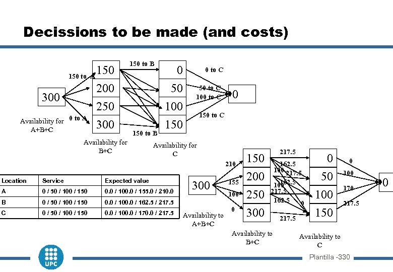
Decissions to be made (and costs) 150 to A 150 to B 50 250 Availability for 0 to A A+B+C 0 to C 200 300 0 100 50 to C 100 to C 300 150 to B Availability for B+C 0 150 to C Availability for C 210 Location Service Expected value A 0 / 50 / 100 / 150 0. 0 / 100. 0 / 155. 0 / 210. 0 B 0 / 50 / 100 / 150 0. 0 / 100. 0 / 162. 5 / 217. 5 C 0 / 50 / 100 / 150 0. 0 / 100. 0 / 170. 0 / 217. 5 300 Availability to A+B+C 155 100 0 150 200 250 300 217. 5 162. 5 100 217. 5 162. 5 0 Availability to B+C 217. 5 0 50 100 150 0 100 170 217. 5 Availability to C Plantilla -330 0

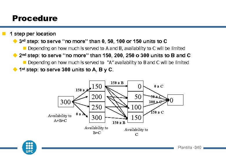
Procedure n 1 step per location u 3 rd step: to serve “no more” than 0, 50, 100 or 150 units to C n Depending on how much is served to A and B, availability to C will be limited u 2 nd step: to serve “no more” than 150, 200, 250 o 300 units to B and C n Depending on how much is served to “A” availability to B and C will be limited u 1 st step: to serve 300 units to A, B y C. Availability to A+B+C 0 a. A 0 a. C 50 250 300 0 200 150 a A 150 a B 100 50 a C 100 a C 300 150 Availability to B+C 150 a B 0 150 a C Availability to C Plantilla -340

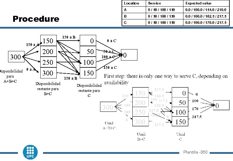
Location 150 a A 300 150 200 250 300 50 a C 100 a C 0 / 50 / 100 / 150 0. 0 / 100. 0 / 162. 5 / 217. 5 0 / 50 / 100 / 150 0. 0 / 100. 0 / 170. 0 / 217. 5 0 a. C 50 100 150 0. 0 / 100. 0 / 155. 0 / 210. 0 C 0 0 / 50 / 100 / 150 B 150 a B Expected value A Procedure Service 0 150 a C Disponibilidad 0 a A para 150 a B A+B+C Disponibilidad restante para B+C C Plantilla -350

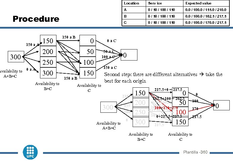
Location Availability to 0 a A A+B+C 0 50 100 50 a C 100 a C 0 / 50 / 100 / 150 0. 0 / 100. 0 / 162. 5 / 217. 5 0 / 50 / 100 / 150 0. 0 / 100. 0 / 170. 0 / 217. 5 0 a. C 250 300 150 0. 0 / 100. 0 / 155. 0 / 210. 0 C 200 150 a A 0 / 50 / 100 / 150 B 150 a B Expected value A Procedure Serv ice 300 Availability to B+C 150 a B 0 150 a C 150 Availability to C Second step: there are different alternatives take the best for each origin 217. 5+0 = 217. 5 210 300 Availability to A+B+C 155 100 0 150 0 162. 5+100 = 262. 5 200 100 217. 5 50 162. 5 100+170=270 Unid 217. 5 250 162. 5 100 B+C 0+217. 5=217. 5 300 217. 5 150 Availability to B+C 0 100 170 217. 5 Availability to C Plantilla -360 0

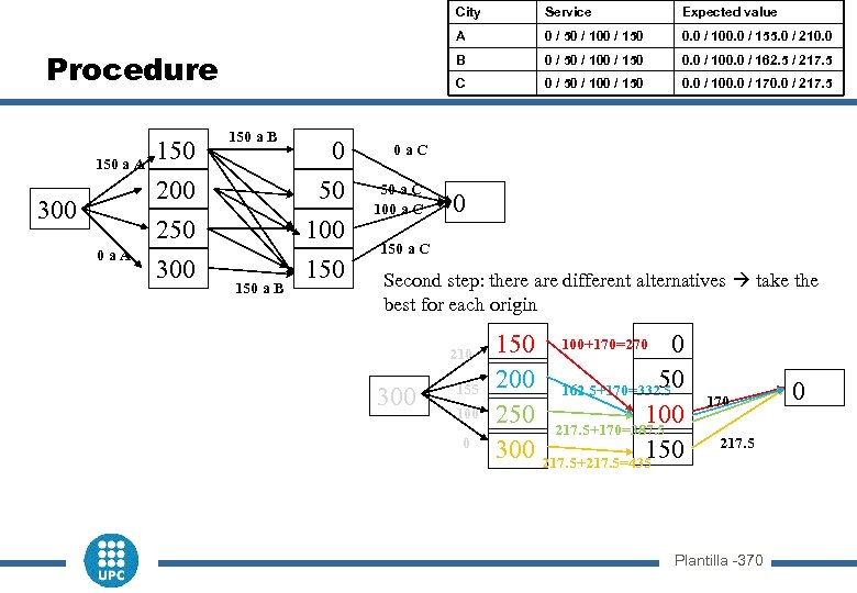
City 150 a A 300 0 a. A 150 200 250 300 150 a B 50 a C 100 a C 0 / 50 / 100 / 150 0. 0 / 100. 0 / 162. 5 / 217. 5 0 / 50 / 100 / 150 0. 0 / 100. 0 / 170. 0 / 217. 5 0 a. C 50 100 150 0. 0 / 100. 0 / 155. 0 / 210. 0 C 0 0 / 50 / 100 / 150 B 150 a B Expected value A Procedure Service 0 150 a C Second step: there are different alternatives take the best for each origin 210 300 155 100 0 150 100+170=270 0 200 162. 5+170=332. 5 50 Unid 100 250 217. 5+170=387. 5 C B+C 300 217. 5+217. 5=435 150 170 217. 5 Plantilla -370 0

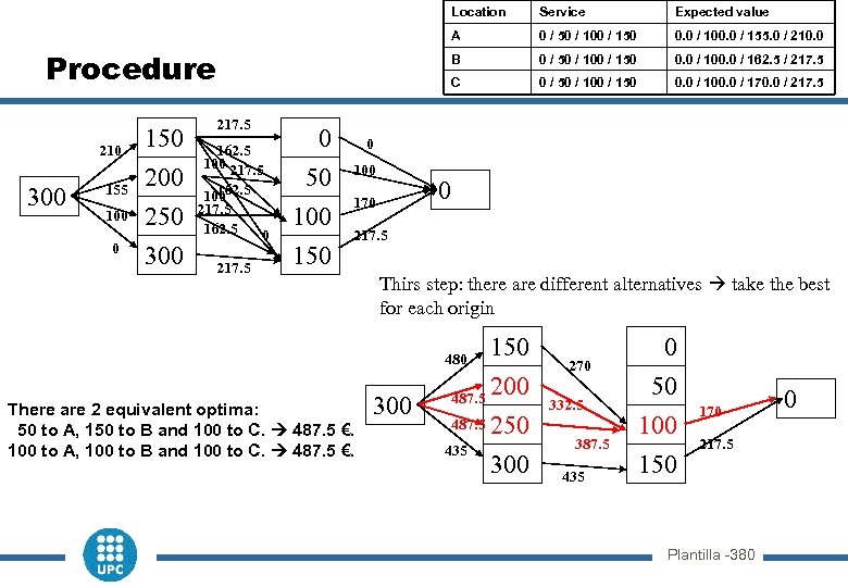
Location 210 300 155 100 0 150 200 250 300 217. 5 0 50 100 150 0. 0 / 100. 0 / 155. 0 / 210. 0 0 / 50 / 100 / 150 0. 0 / 100. 0 / 162. 5 / 217. 5 C 162. 5 100 217. 5 162. 5 0 0 / 50 / 100 / 150 B 217. 5 Expected value A Procedure Service 0 / 50 / 100 / 150 0. 0 / 100. 0 / 170. 0 / 217. 5 0 100 0 170 217. 5 Thirs step: there are different alternatives take the best for each origin 150 200 487. 5 Unid B+C 487. 5 250 435 300 480 There are 2 equivalent optima: 50 to A, 150 to B and 100 to C. 487. 5 €. 100 to A, 100 to B and 100 to C. 487. 5 €. 300 270 332. 5 387. 5 435 0 50 100 150 170 217. 5 Plantilla -380 0

Limitations: what else ? n Uncertainty modeling u Fuzzy sets ? Fuzzy programming ? (principle of “difficulty conservation”? ) n Generalization of methodologies (modeling and solution) u Multiple sources of uncertainty u Multiple objectives ( “trade off”) n Computing efficiency (industrial problem) n Uncertainty of uncertainty Plantilla -390