Value at Risk VAR VAR is the maximum

Value at Risk (VAR) VAR is the maximum loss over a target horizon within a confidence interval (or, under normal market conditions) In other words, if none of the “extreme events” (i. e. , low-probability events) occurs, what is my maximum loss over a given time period?

Another Definition of VAR • A forecast of a given percentile, usually in the lower tail, of the distribution of returns on a portfolio over some period; similar in principle to an estimate of the expected return on a portfolio, which is a forecast of the 50 th percentile. Ex: 95% one-tail normal distribution is 1. 645 sigma (Pr(x<=X)=0. 05, X=-1. 645) while 99% normal distribution is 2. 326 sigma

VAR: Example • Consider a $100 million portfolio of medium-term bonds. Suppose my confidence interval is 95% (i. e. , 95% of possible market events is defined as “normal”. ) Then, what is the maximum monthly loss under normal markets over any month? • To answer this question, let’s look at the monthly medium-term bond returns from 1953 to 1995: • Lowest: -6. 5% vs. Highest: 12%

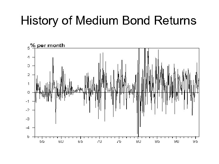History of Medium Bond Returns

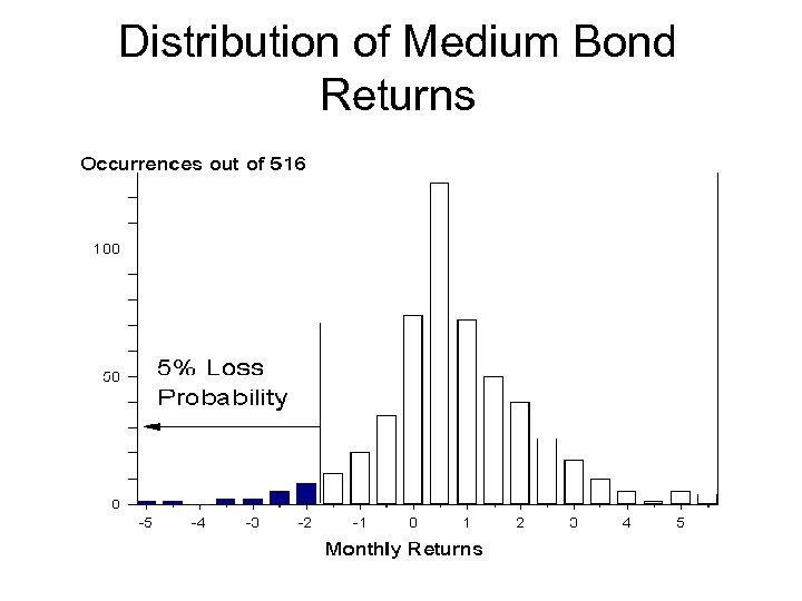Distribution of Medium Bond Returns

Calculating VAR at 95% Confidence • At the 95% confidence interval, the lowest monthly return is -1. 7%. (I. e. , there is a 5% chance that the monthly medium bond return is lower than -1. 7%) That is, there are 26 months out of the 516 for which the monthly returns were lower than -1. 7%. • VAR = 100 million X 1. 7% = $1. 7 million • (95% of the time, the portfolio’s loss will be no more than $1. 7 million!)

Issues to Ponder • What horizon is appropriate? A day, a month, or a year? the holding period should correspond to the longest period needed for an orderly portfolio liquidation. • • What confidence level to consider? * Are you risk averse? The more risk averse => (1) the higher confidence level necessary & (2) the lower VAR desired.

How to convert Va. R parameters If Assuming normal distribution and since returns are uncorrelated day-to-day: • VAR(T days) = VAR(1 day) x SQRT(T) And 95% one-tail Va. R corresponds to 1. 645 of sigma while 99% Va. R corresponds to 2. 326 sigma: • VAR(95%) = VAR(99%) x 1. 645 / 2. 326

Va. R Computation • Parametric: Delta-Normal Portfolio return is normally distributed as it is the linear combination of risky assets, therefore need: 1. predicted variances and correlations of each asset (going back 5 years), no need for returns data. 2. Position on each asset (risk factor).

Va. R Computation-continued • Historical simulation going back in time, e. g. over the last 5 years, and applying current weights to a time-series of historical asset returns. This return does not represent an actual portfolio but rather reconstructs the history of a hypothetical portfolio using the current position • (1) for each risk factor, a time-series of actual movements, and • (2) positions on risk factors.

Va. R Computation-continued Monte Carlo Simulation two steps: • Specifies a stochastic process for financial variables as well as process parameters; the choice of distributions and parameters such as risk and correlations can be derived from historical data. • Fictitious price paths are simulated for all variables of interest. At each horizon considered, one day to many months ahead, the portfolio is marked-to-market using full valuation. Each of these ``pseudo'' realizations is then used to compile a distribution of returns, from which a VAR figure can be measured. Required: • for each risk factor, specification of a stochastic process (i. e. , distribution and parameters), • valuation models for all assets in the portfolio, and • positions on various securities.

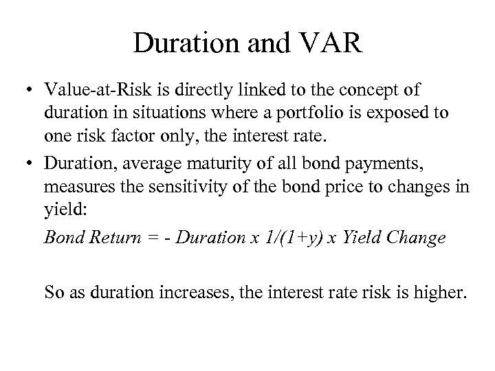Duration and VAR • Value-at-Risk is directly linked to the concept of duration in situations where a portfolio is exposed to one risk factor only, the interest rate. • Duration, average maturity of all bond payments, measures the sensitivity of the bond price to changes in yield: Bond Return = - Duration x 1/(1+y) x Yield Change So as duration increases, the interest rate risk is higher.

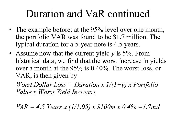Duration and Va. R continued • The example before: at the 95% level over one month, the portfolio VAR was found to be $1. 7 million. The typical duration for a 5 -year note is 4. 5 years. • Assume now that the current yield y is 5%. From historical data, we find that the worst increase in yields over a month at the 95% is 0. 40%. The worst loss, or VAR, is then given by Worst Dollar Loss = Duration x 1/(1+y) x Portfolio Value x Worst Yield Increase VAR = 4. 5 Years x (1/1. 05) x $100 m x 0. 4% =1. 7 mil

Va. R in practice • J. P. Morgan Riskmetrics allows users to compute a portfolio VAR using the Delta-Normal method based on a 95% confidence level over a daily or monthly horizon • Deutsche Bank, RAROC 2020 system provides VAR estimates at the 99% level of confidence over an annual horizon, using the Monte Carlo method.

Weaknesses • Va. R does not measure "event" (e. g. , market crash) risk. That is why portfolio stress tests are recommended to supplement Va. R. • Va. R does not readily capture liquidity differences among instruments. That is why limits on both tenors and option greeks are still useful. • Va. R doesn't readily capture model risks, which is why model reserves are also necessary.

Question • What are the methods to calculate Va. R?