1424a633642e817f5e5853e9d349da11.ppt
- Количество слайдов: 22
Valuation of Non-Market Goods • Normally, in CBA, use CS or WTP to measure benefits
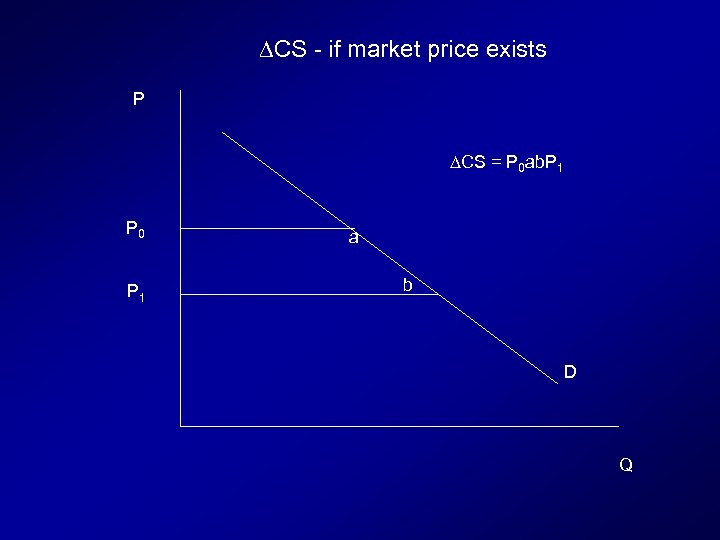
∆CS - if market price exists P ∆CS = P 0 ab. P 1 P 0 P 1 a b D Q
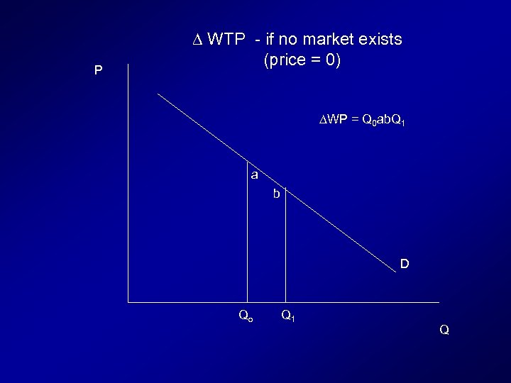
P ∆ WTP - if no market exists (price = 0) WP = Q 0 ab. Q 1 a b D Qo Q 1 Q
Valuation of Non-Market Goods • What to do if a project provides a good or service for which there is no market? – No market price – No market demand curve – Cannot measure changes in WTP or CS
Valuation of Non-Market Goods • A number of CBA techniques have been developed to estimate WTP for nonmarketed goods and services • “Revealed Preference Methods” Boardman et al. , Chapter 13 – See also Zerbe & Dively, Chapter 18
Valuation of Non-Market Goods • Some techniques: – Markets for substitute goods (analogous goods) – Hedonic pricing – Cost savings and intermediate goods – Travel Cost
Substitutes • Public sector provides a good or service that is identical to what is provided by private sector: – Housing – Medical services – Schools
Substitutes • But what if the project is not providing a good or service that is not identical (not a perfect substitute) of what private market provides? • E. g. public housing is low-cost housing in areas with lower property values. • Use hedonic pricing technique
Hedonic Pricing • View demand as implicit demand for a bundle of implicit characteristics that are bound together within a good or service • Price of house = f(#BR, Sq. ft, lot size, school quality, distance to shopping areas, noise level, crime rate, …. . ) • Collect information from a sample of households with different characteristics of these characteristics
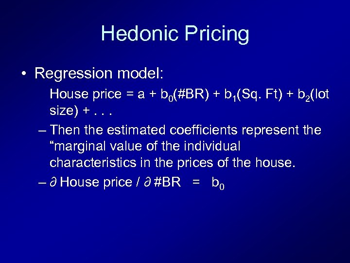
Hedonic Pricing • Regression model: House price = a + b 0(#BR) + b 1(Sq. Ft) + b 2(lot size) +. . . – Then the estimated coefficients represent the “marginal value of the individual characteristics in the prices of the house. – ∂ House price / ∂ #BR = b 0
Hedonic Pricing • With this information can estimate the value of houses with particular characteristics, in particular locations. • Projects may also change some of the individual characteristics, and the estimated coefficients can be used to value project outputs • Estimate the amount that reducing noise level in neighborhood around airport will increase home values in the neighborhood.
Intermediate goods (inputs) • Theoretically, can use derived demand curve (market demand for the input) to measure changes in WTP, CS • Often there is not an existing market for the input – If the project is providing the input for the first time
Intermediate Goods • Estimate: Income with project – Income without project • Example – impact of irrigation project – Estimate farmers’ income with irrigation water with income without irrigation • • Higher yields, changed cropping patterns Before/after comparisons Returns from farmers in existing irrigated regions In both cases, problem of attributing measured differences to only the availability of irrigation water
Intermediate Goods • In this simple example, assume constant marginal product of water. – Do not measure the incremental profit from each additional unit of water available – Reasonable assumption for small projects, possible less reasonable for large projects
Travel Cost • Often used to measure the value of recreational sites – Users must travel to get to site – This travel is part of the “price” of using the site – Different users have different travel costs, and so pay different “prices” – Assume all consumers (users) have same preferences, – Then differences in the observed use levels (visits) can be associated with different “prices” to estimate WTP of the “representative” consumer
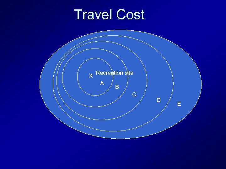
Travel Cost X Recreation site A D B C D E
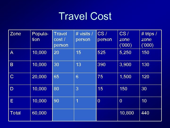
Travel Cost Zone Population Travel cost / person # visits / person CS / zone (‘ 000) # trips / zone (’ 000) A 10, 000 20 15 525 5, 250 150 B 10, 000 30 13 390 3, 900 130 C 20, 000 65 6 75 1, 500 120 D 10, 000 80 3 15 150 30 E 10, 000 90 1 0 0 10 Total 60, 000 10, 800 440
Travel Cost • From this information can derive market “demand” curve • Spreadsheet
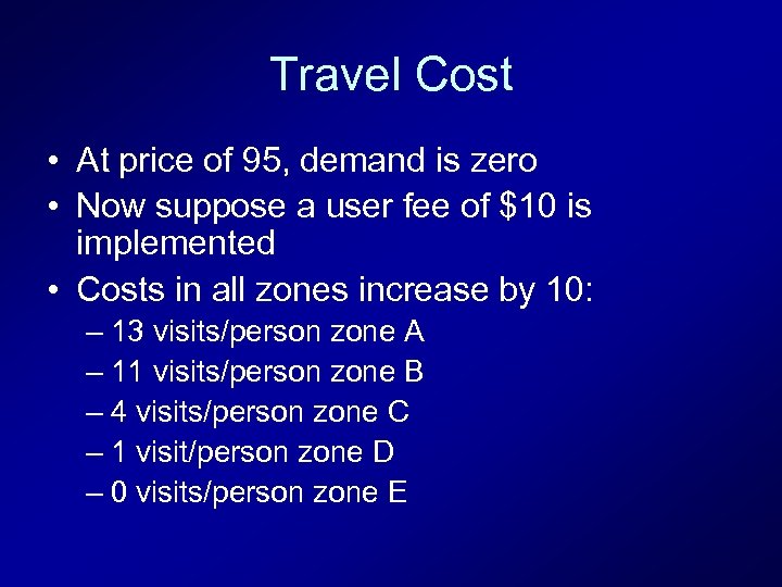
Travel Cost • At price of 95, demand is zero • Now suppose a user fee of $10 is implemented • Costs in all zones increase by 10: – 13 visits/person zone A – 11 visits/person zone B – 4 visits/person zone C – 1 visit/person zone D – 0 visits/person zone E
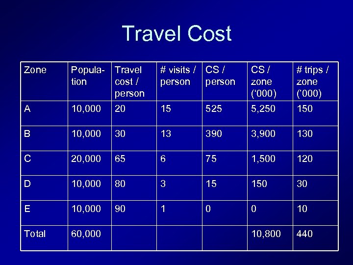
Travel Cost Zone Population Travel cost / person # visits / person CS / zone (‘ 000) # trips / zone (’ 000) A 10, 000 20 15 525 5, 250 150 B 10, 000 30 13 390 3, 900 130 C 20, 000 65 6 75 1, 500 120 D 10, 000 80 3 15 150 30 E 10, 000 90 1 0 0 10 Total 60, 000 10, 800 440
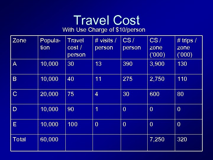
Travel Cost With Use Charge of $10/person Zone Population Travel cost / person # visits / person CS / zone (‘ 000) # trips / zone (’ 000) A 10, 000 30 13 390 3, 900 130 B 10, 000 40 11 275 2, 750 110 C 20, 000 75 4 30 600 80 D 10, 000 90 1 0 0 0 E 10, 000 100 0 0 Total 60, 000 7, 250 320
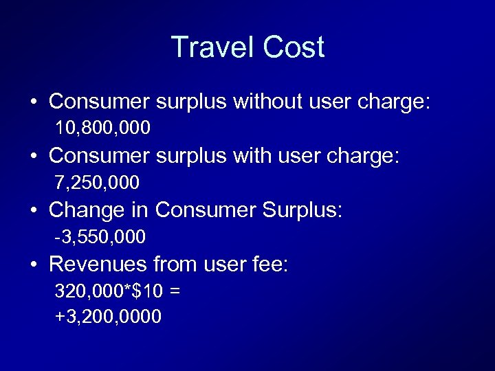
Travel Cost • Consumer surplus without user charge: 10, 800, 000 • Consumer surplus with user charge: 7, 250, 000 • Change in Consumer Surplus: -3, 550, 000 • Revenues from user fee: 320, 000*$10 = +3, 200, 0000
1424a633642e817f5e5853e9d349da11.ppt