V 1 Introduction Mon Oct 14 2013

V 1 – Introduction Mon, Oct 14, 2013 Bioinformatics 3 — Volkhard Helms

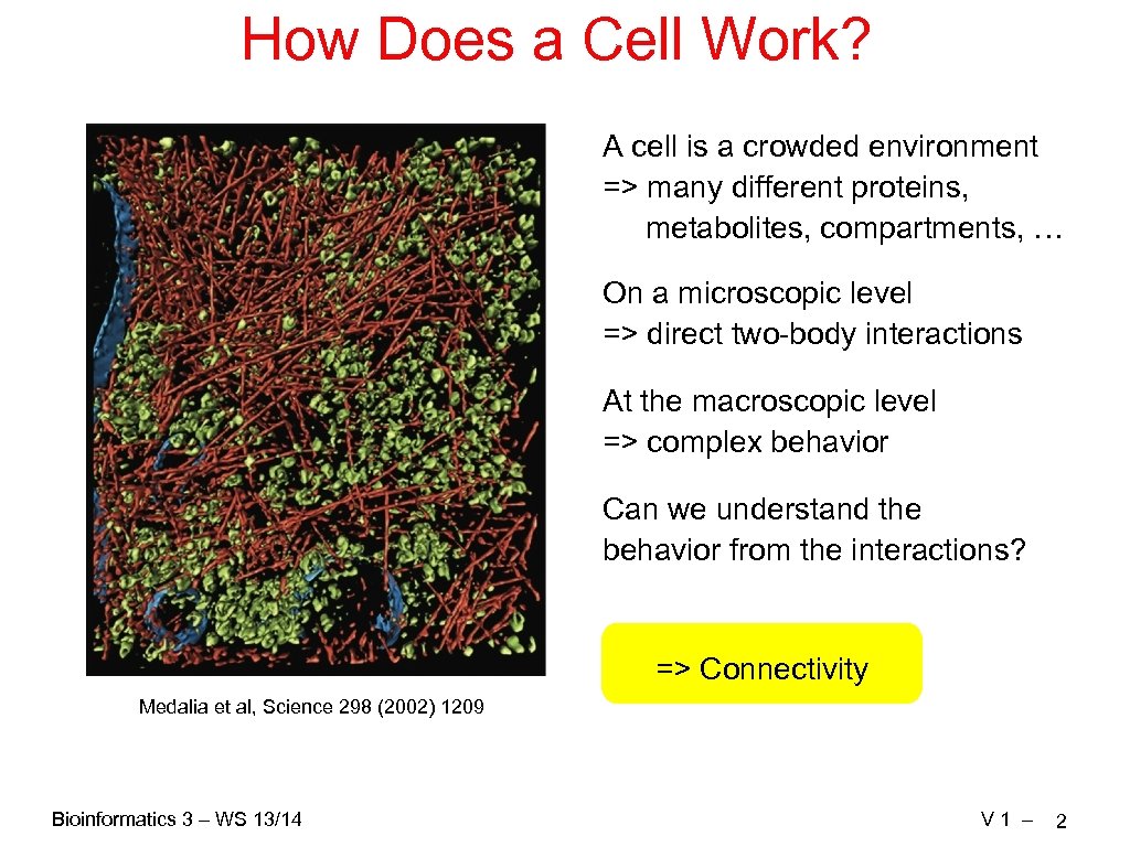How Does a Cell Work? A cell is a crowded environment => many different proteins, metabolites, compartments, … On a microscopic level => direct two-body interactions At the macroscopic level => complex behavior Can we understand the behavior from the interactions? => Connectivity Medalia et al, Science 298 (2002) 1209 Bioinformatics 3 – WS 13/14 V 1 – 2

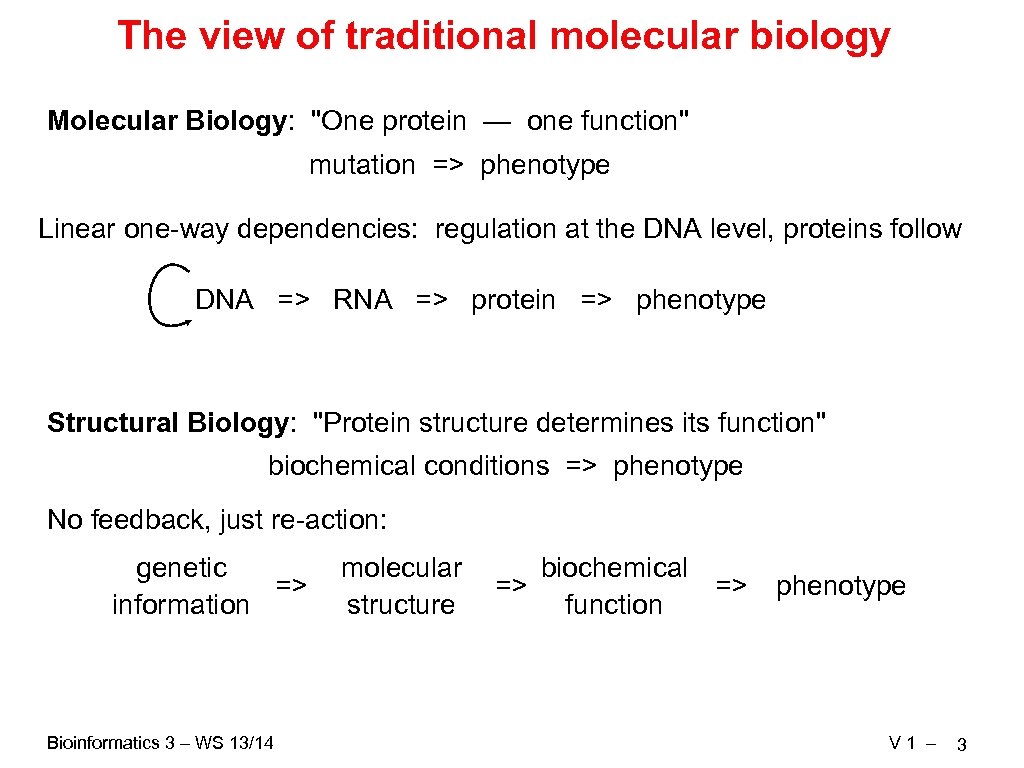The view of traditional molecular biology Molecular Biology: "One protein — one function" mutation => phenotype Linear one-way dependencies: regulation at the DNA level, proteins follow DNA => RNA => protein => phenotype Structural Biology: "Protein structure determines its function" biochemical conditions => phenotype No feedback, just re-action: genetic => information Bioinformatics 3 – WS 13/14 molecular structure biochemical => => function phenotype V 1 – 3

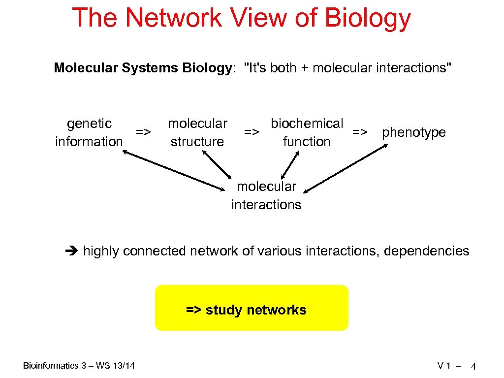The Network View of Biology Molecular Systems Biology: "It's both + molecular interactions" genetic => information molecular structure biochemical => => function phenotype molecular interactions highly connected network of various interactions, dependencies => study networks Bioinformatics 3 – WS 13/14 V 1 – 4

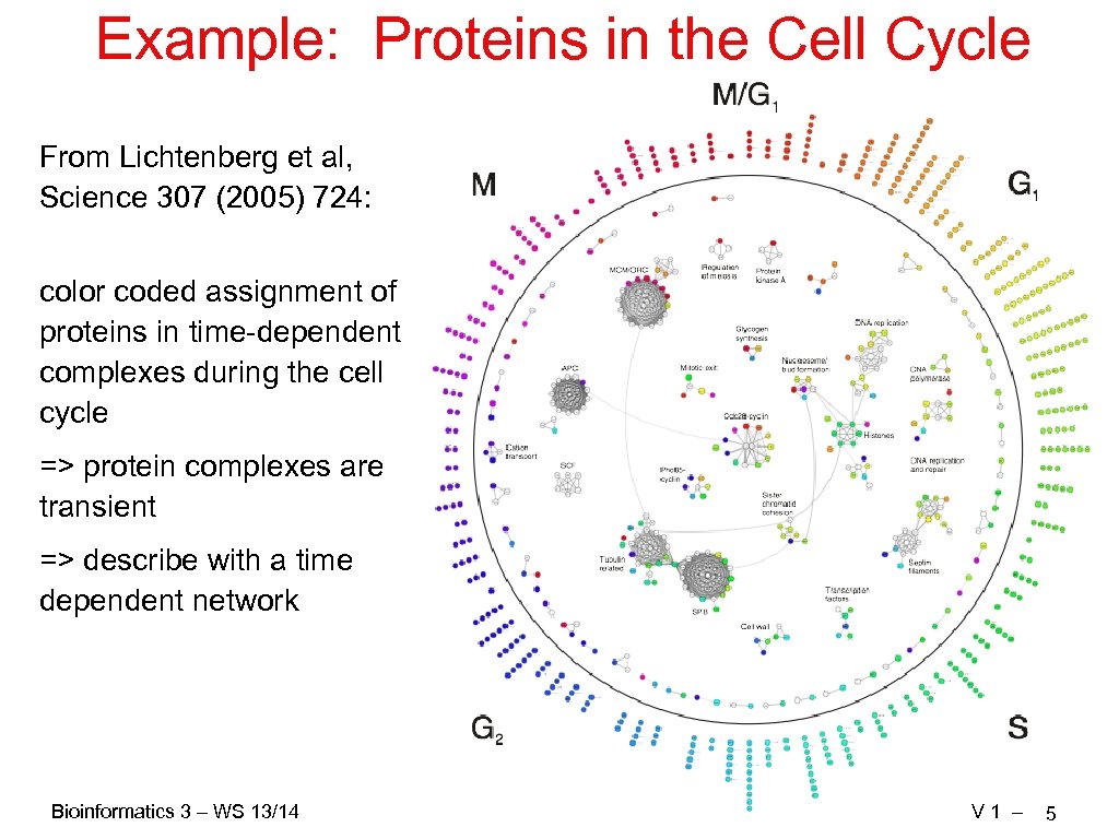Example: Proteins in the Cell Cycle From Lichtenberg et al, Science 307 (2005) 724: color coded assignment of proteins in time-dependent complexes during the cell cycle => protein complexes are transient => describe with a time dependent network Bioinformatics 3 – WS 13/14 V 1 – 5

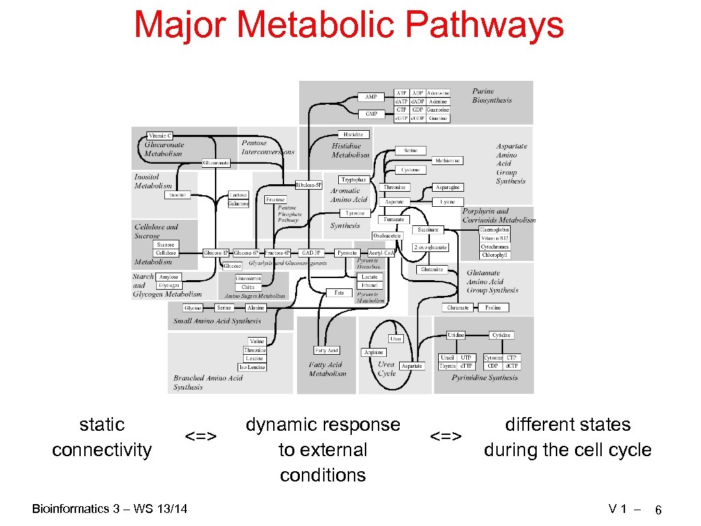Major Metabolic Pathways static connectivity <=> Bioinformatics 3 – WS 13/14 dynamic response to external conditions <=> different states during the cell cycle V 1 – 6

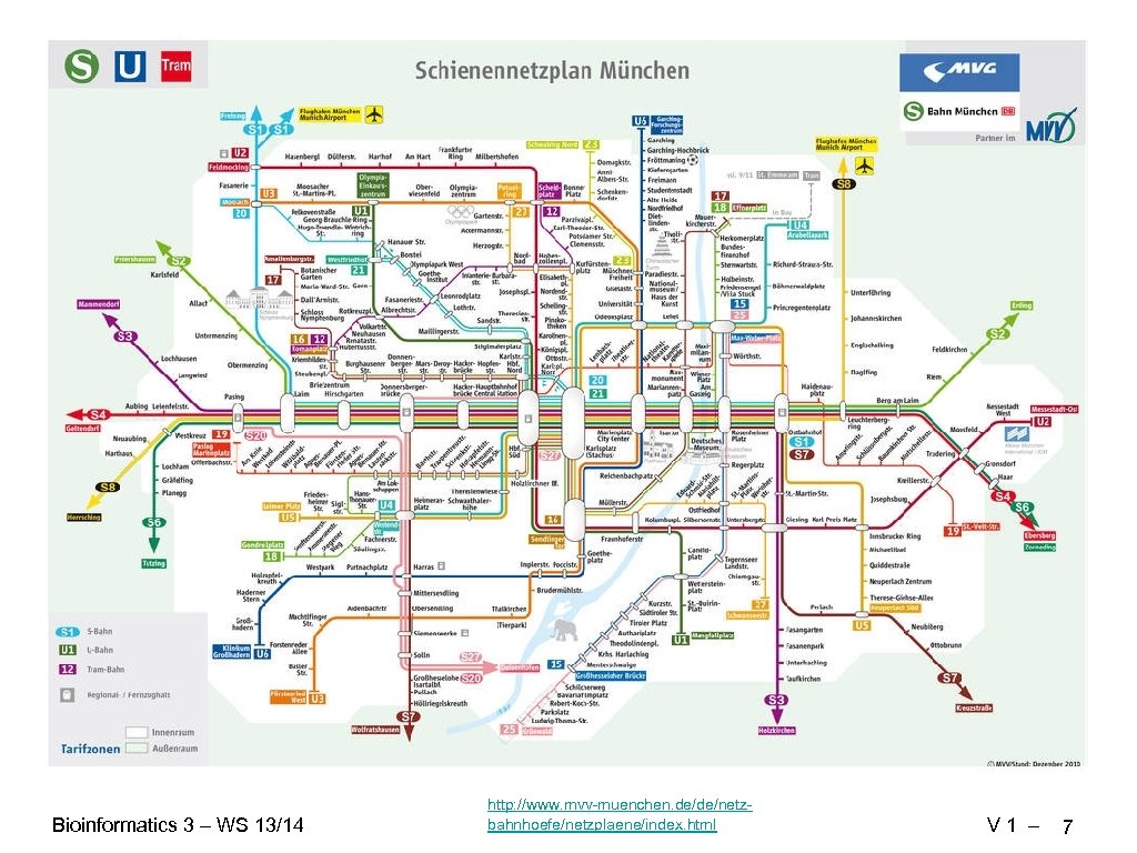Bioinformatics 3 – WS 13/14 http: //www. mvv-muenchen. de/de/netzbahnhoefe/netzplaene/index. html V 1 – 7

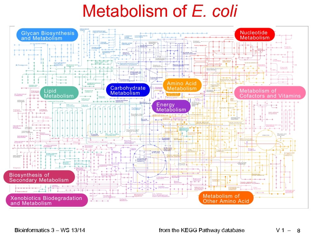Metabolism of E. coli Bioinformatics 3 – WS 13/14 from the KEGG Pathway database V 1 – 8

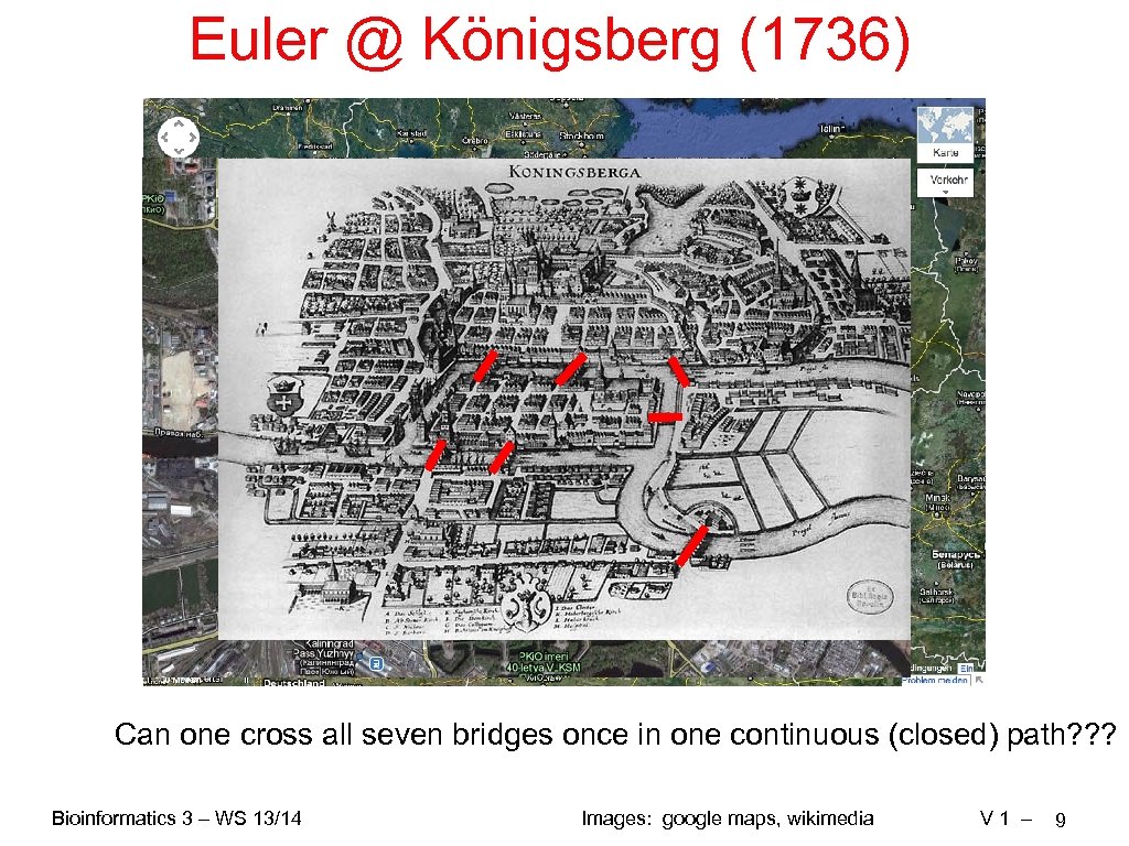Euler @ Königsberg (1736) Can one cross all seven bridges once in one continuous (closed) path? ? ? Bioinformatics 3 – WS 13/14 Images: google maps, wikimedia V 1 – 9

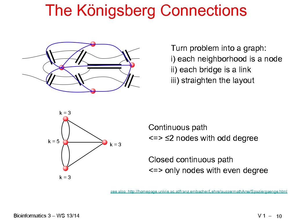The Königsberg Connections Turn problem into a graph: i) each neighborhood is a node ii) each bridge is a link iii) straighten the layout k=3 k=5 k=3 Continuous path <=> ≤ 2 nodes with odd degree Closed continuous path <=> only nodes with even degree see also: http: //homepage. univie. ac. at/franz. embacher/Lehre/aussermath. Anw/Spaziergaenge. html Bioinformatics 3 – WS 13/14 V 1 – 10

size of" src="https://present5.com/presentation/eb01d272bb34ff70ffa4be780b9d7464/image-11.jpg" alt="Quantify the "Hairy Monsters" Network Measures: • No. of edges, nodes => size of" /> Quantify the "Hairy Monsters" Network Measures: • No. of edges, nodes => size of the network • Average degree => density of connections • Degree distribution P(k) => structure of the network • Cluster coefficient C(k) => local connectivity • Connected components => subgraphs Schwikowski, Uetz, Fields, Nature Biotech. 18, 1257 (2001) Bioinformatics 3 – WS 13/14 V 1 – 11

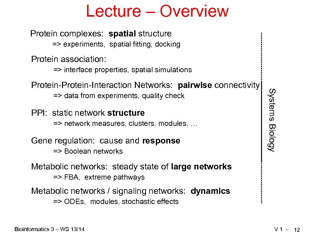Lecture – Overview Protein complexes: spatial structure => experiments, spatial fitting, docking Protein association: => interface properties, spatial simulations => data from experiments, quality check PPI: static network structure => network measures, clusters, modules, … Gene regulation: cause and response => Boolean networks Systems Biology Protein-Interaction Networks: pairwise connectivity Metabolic networks: steady state of large networks => FBA, extreme pathways Metabolic networks / signaling networks: dynamics => ODEs, modules, stochastic effects Bioinformatics 3 – WS 13/14 V 1 – 12

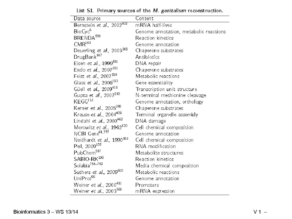
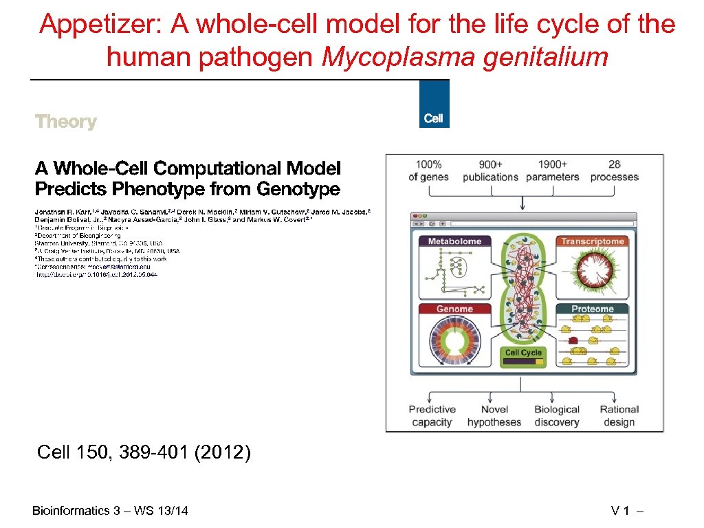Appetizer: A whole-cell model for the life cycle of the human pathogen Mycoplasma genitalium Cell 150, 389 -401 (2012) Bioinformatics 3 – WS 13/14 V 1 –

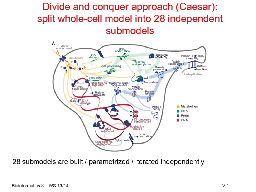Divide and conquer approach (Caesar): split whole-cell model into 28 independent submodels 28 submodels are built / parametrized / iterated independently Bioinformatics 3 – WS 13/14 V 1 –

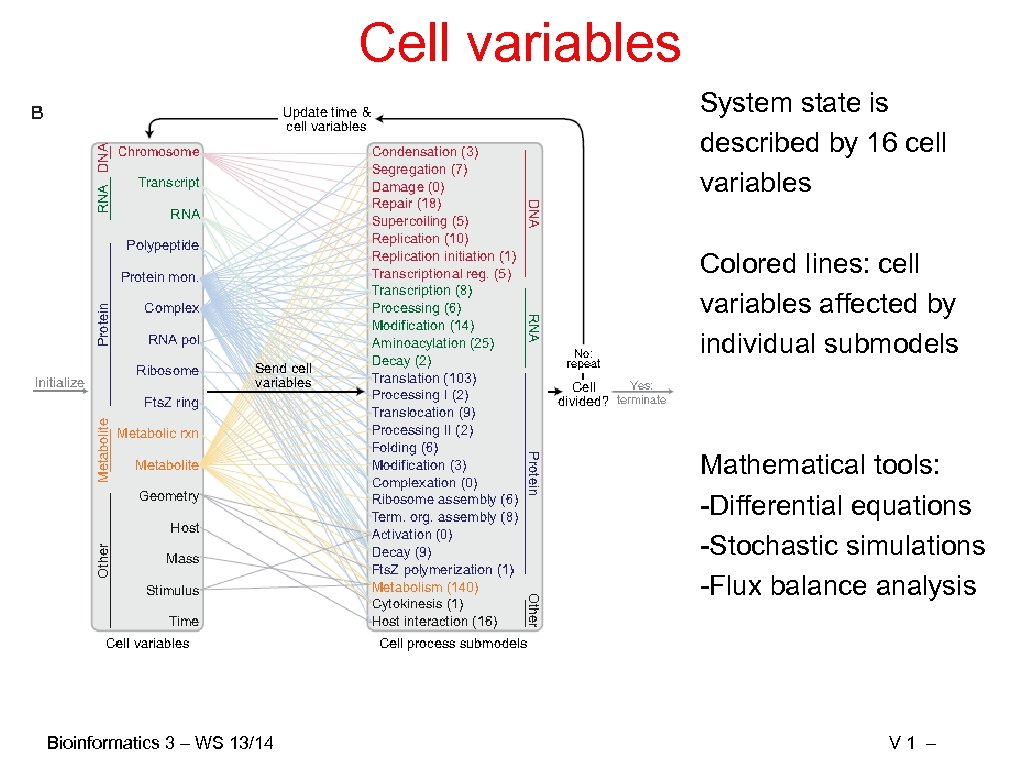Cell variables System state is described by 16 cell variables Colored lines: cell variables affected by individual submodels Mathematical tools: -Differential equations -Stochastic simulations -Flux balance analysis Bioinformatics 3 – WS 13/14 V 1 –

Bioinformatics 3 – WS 13/14 V 1 –

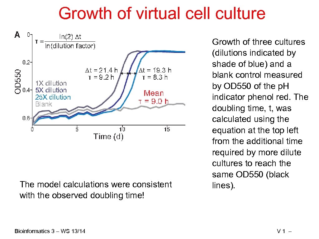Growth of virtual cell culture The model calculations were consistent with the observed doubling time! Bioinformatics 3 – WS 13/14 Growth of three cultures (dilutions indicated by shade of blue) and a blank control measured by OD 550 of the p. H indicator phenol red. The doubling time, t, was calculated using the equation at the top left from the additional time required by more dilute cultures to reach the same OD 550 (black lines). V 1 –

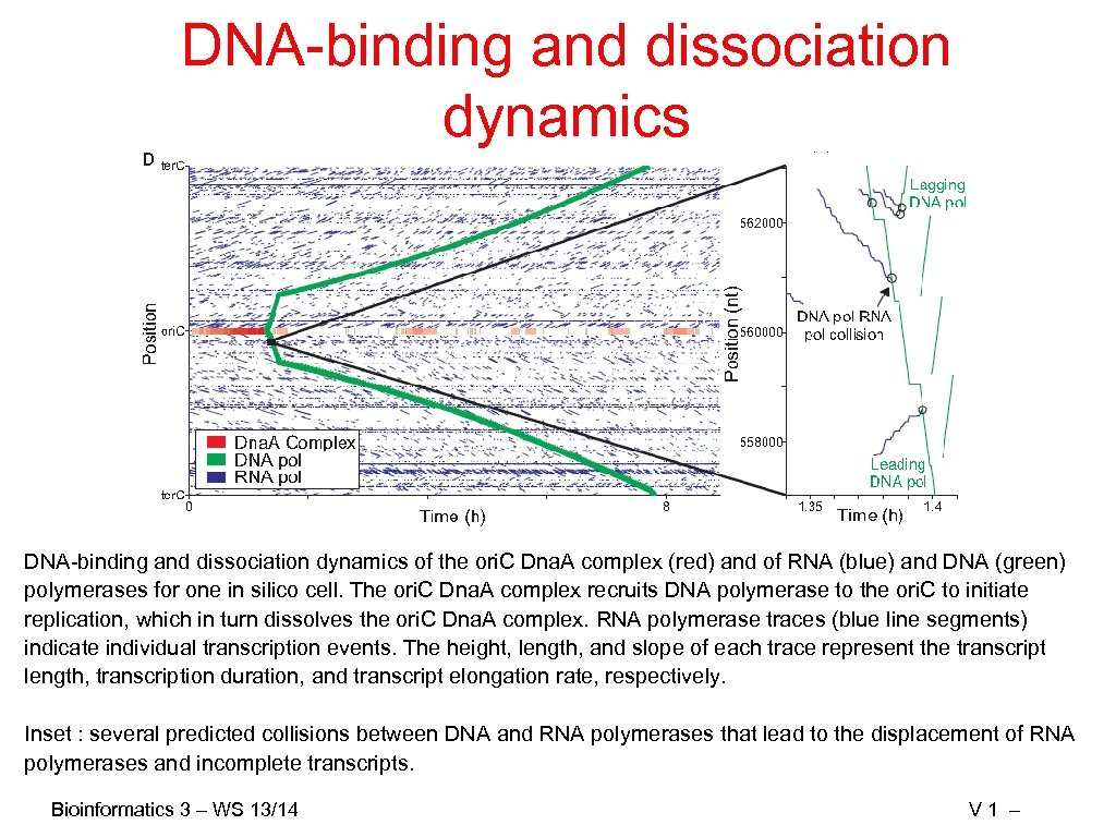DNA-binding and dissociation dynamics of the ori. C Dna. A complex (red) and of RNA (blue) and DNA (green) polymerases for one in silico cell. The ori. C Dna. A complex recruits DNA polymerase to the ori. C to initiate replication, which in turn dissolves the ori. C Dna. A complex. RNA polymerase traces (blue line segments) indicate individual transcription events. The height, length, and slope of each trace represent the transcript length, transcription duration, and transcript elongation rate, respectively. Inset : several predicted collisions between DNA and RNA polymerases that lead to the displacement of RNA polymerases and incomplete transcripts. Bioinformatics 3 – WS 13/14 V 1 –

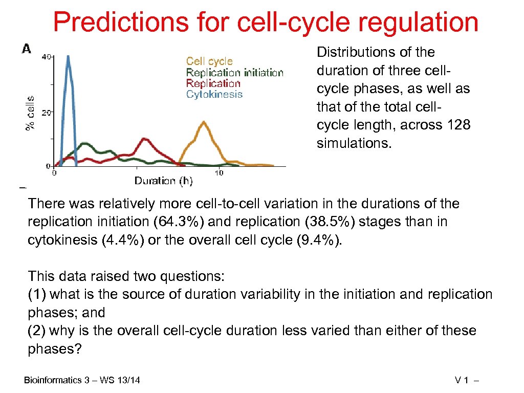Predictions for cell-cycle regulation Distributions of the duration of three cellcycle phases, as well as that of the total cellcycle length, across 128 simulations. There was relatively more cell-to-cell variation in the durations of the replication initiation (64. 3%) and replication (38. 5%) stages than in cytokinesis (4. 4%) or the overall cell cycle (9. 4%). This data raised two questions: (1) what is the source of duration variability in the initiation and replication phases; and (2) why is the overall cell-cycle duration less varied than either of these phases? Bioinformatics 3 – WS 13/14 V 1 –

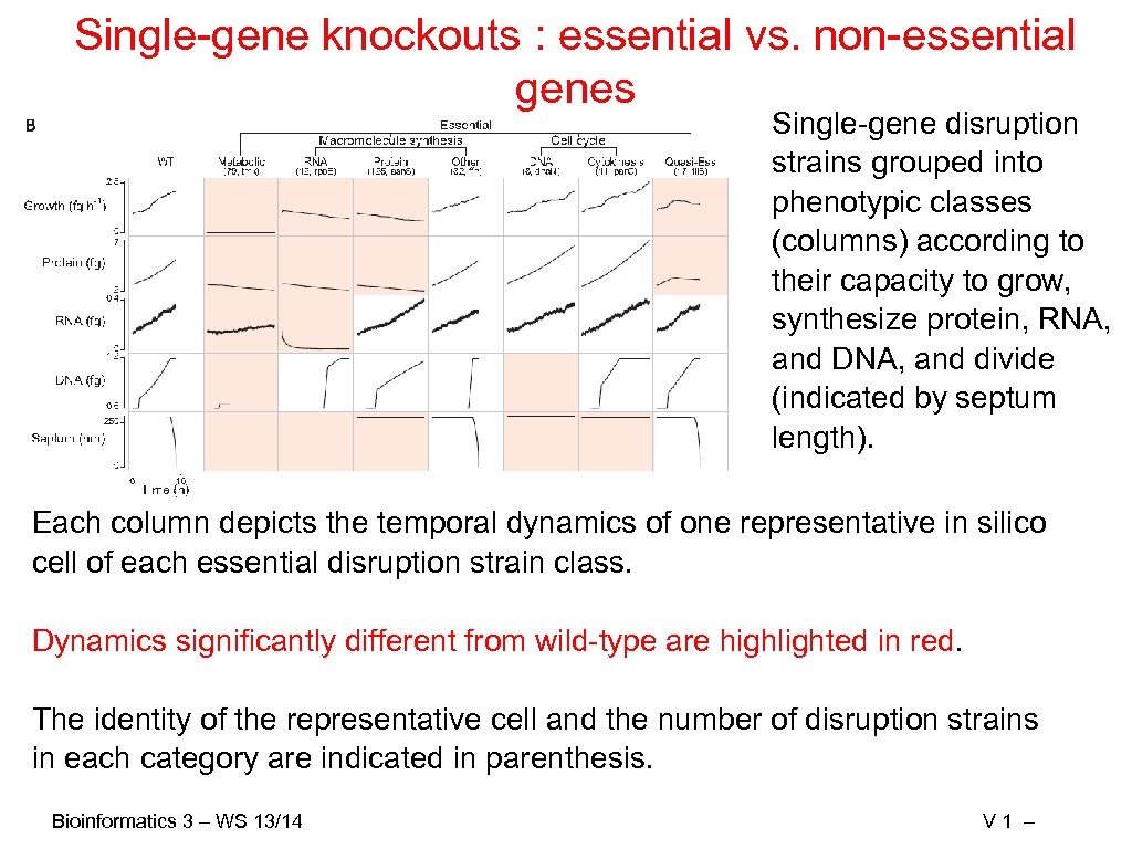Single-gene knockouts : essential vs. non-essential genes Single-gene disruption strains grouped into phenotypic classes (columns) according to their capacity to grow, synthesize protein, RNA, and DNA, and divide (indicated by septum length). Each column depicts the temporal dynamics of one representative in silico cell of each essential disruption strain class. Dynamics significantly different from wild-type are highlighted in red. The identity of the representative cell and the number of disruption strains in each category are indicated in parenthesis. Bioinformatics 3 – WS 13/14 V 1 –

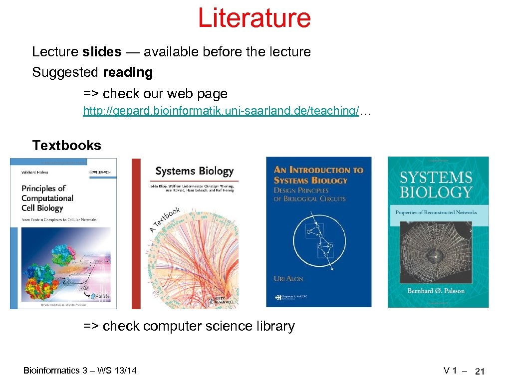Literature Lecture slides — available before the lecture Suggested reading => check our web page http: //gepard. bioinformatik. uni-saarland. de/teaching/… Textbooks => check computer science library Bioinformatics 3 – WS 13/14 V 1 – 21

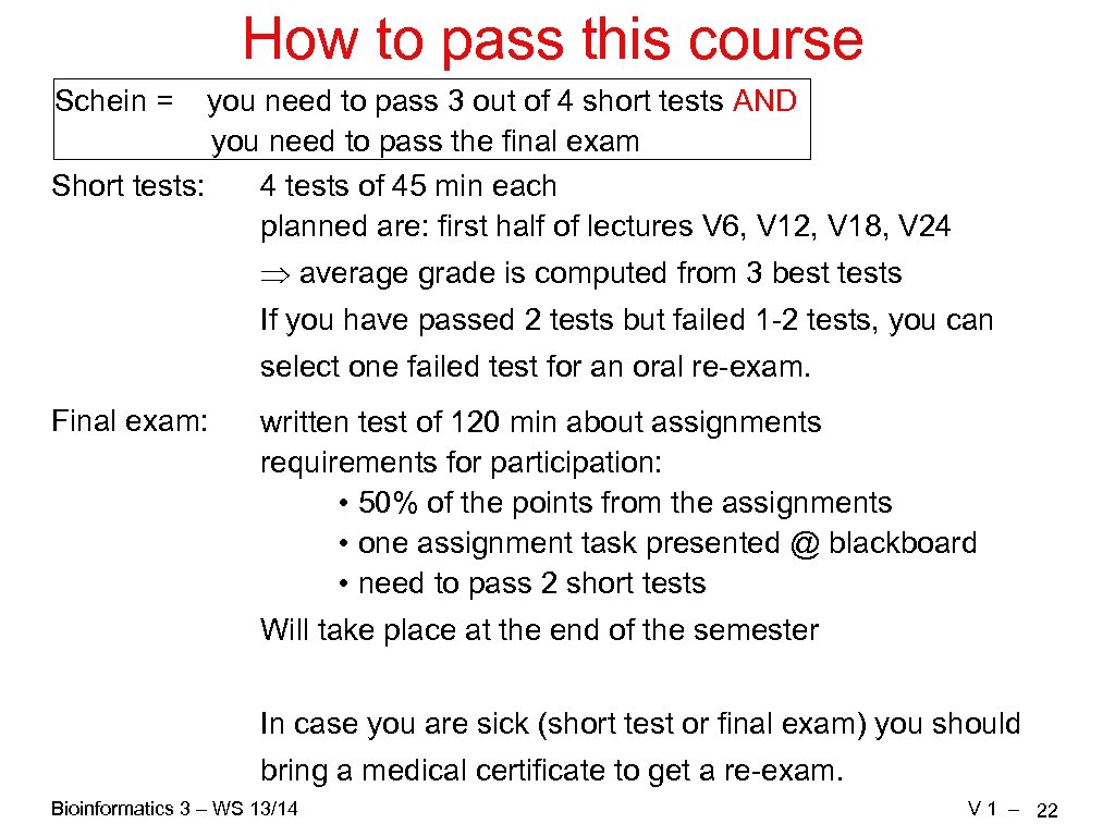How to pass this course Schein = you need to pass 3 out of 4 short tests AND you need to pass the final exam Short tests: 4 tests of 45 min each planned are: first half of lectures V 6, V 12, V 18, V 24 Þ average grade is computed from 3 best tests If you have passed 2 tests but failed 1 -2 tests, you can select one failed test for an oral re-exam. Final exam: written test of 120 min about assignments requirements for participation: • 50% of the points from the assignments • one assignment task presented @ blackboard • need to pass 2 short tests Will take place at the end of the semester In case you are sick (short test or final exam) you should bring a medical certificate to get a re-exam. Bioinformatics 3 – WS 13/14 V 1 – 22

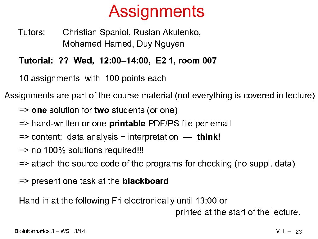Assignments Tutors: Christian Spaniol, Ruslan Akulenko, Mohamed Hamed, Duy Nguyen Tutorial: ? ? Wed, 12: 00– 14: 00, E 2 1, room 007 10 assignments with 100 points each Assignments are part of the course material (not everything is covered in lecture) => one solution for two students (or one) => hand-written or one printable PDF/PS file per email => content: data analysis + interpretation — think! => no 100% solutions required!!! => attach the source code of the programs for checking (no suppl. data) => present one task at the blackboard Hand in at the following Fri electronically until 13: 00 or printed at the start of the lecture. Bioinformatics 3 – WS 13/14 V 1 – 23

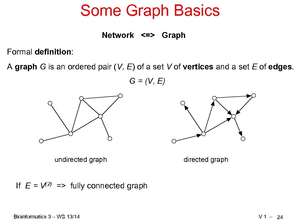Some Graph Basics Network <=> Graph Formal definition: A graph G is an ordered pair (V, E) of a set V of vertices and a set E of edges. G = (V, E) undirected graph If E = V(2) => fully connected graph Bioinformatics 3 – WS 13/14 V 1 – 24

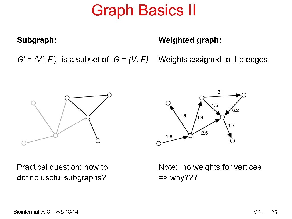Graph Basics II Subgraph: Weighted graph: G' = (V', E') is a subset of G = (V, E) Weights assigned to the edges Practical question: how to define useful subgraphs? Note: no weights for vertices => why? ? ? Bioinformatics 3 – WS 13/14 V 1 – 25

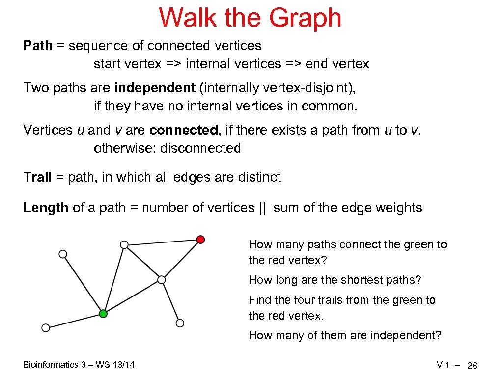Walk the Graph Path = sequence of connected vertices start vertex => internal vertices => end vertex Two paths are independent (internally vertex-disjoint), if they have no internal vertices in common. Vertices u and v are connected, if there exists a path from u to v. otherwise: disconnected Trail = path, in which all edges are distinct Length of a path = number of vertices || sum of the edge weights How many paths connect the green to the red vertex? How long are the shortest paths? Find the four trails from the green to the red vertex. How many of them are independent? Bioinformatics 3 – WS 13/14 V 1 – 26

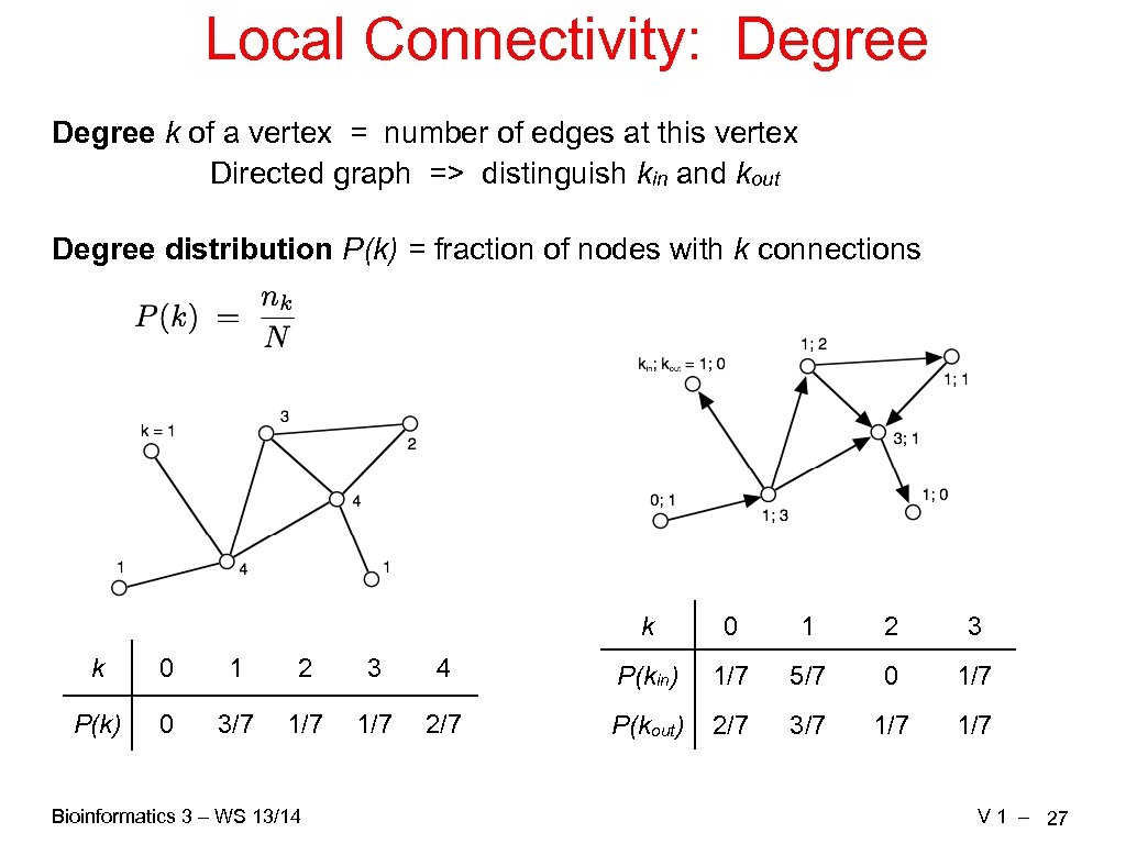Local Connectivity: Degree k of a vertex = number of edges at this vertex Directed graph => distinguish kin and kout Degree distribution P(k) = fraction of nodes with k connections k 0 1 2 3 4 P(kin) 1/7 5/7 0 1/7 P(k) 0 3/7 1/7 2/7 P(kout) 2/7 3/7 1/7 Bioinformatics 3 – WS 13/14 V 1 – 27

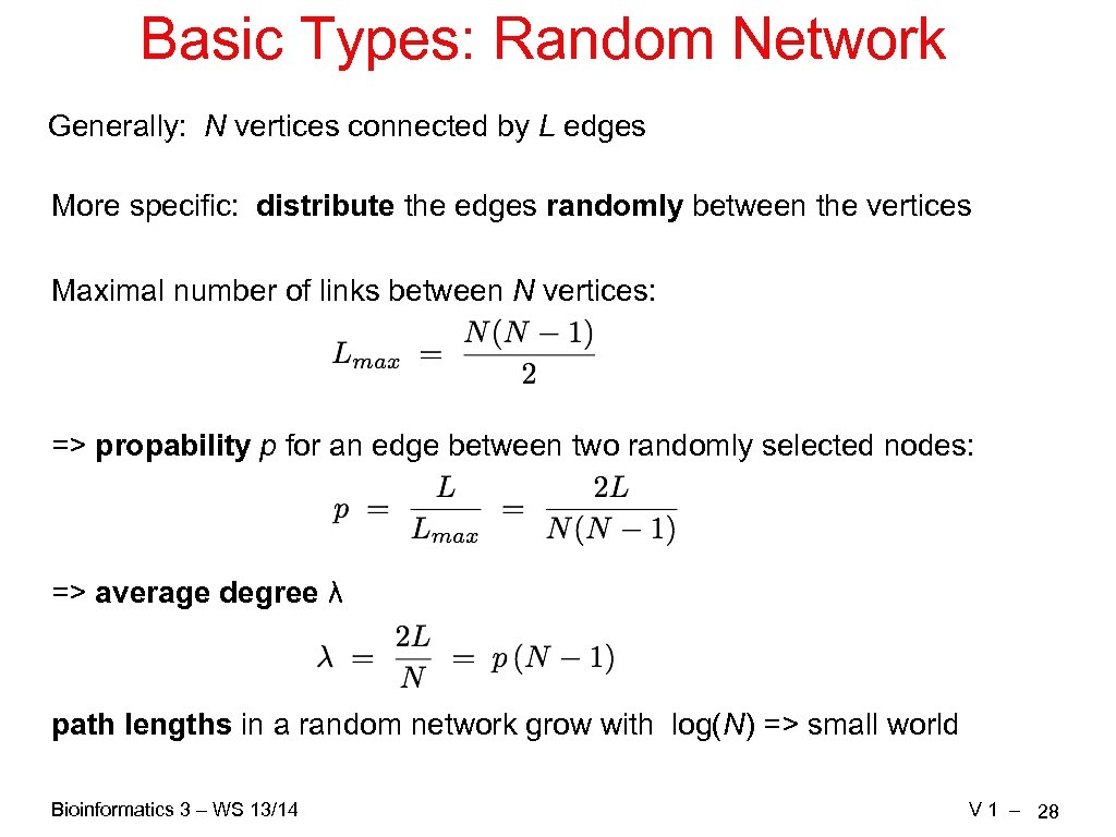Basic Types: Random Network Generally: N vertices connected by L edges More specific: distribute the edges randomly between the vertices Maximal number of links between N vertices: => propability p for an edge between two randomly selected nodes: => average degree λ path lengths in a random network grow with log(N) => small world Bioinformatics 3 – WS 13/14 V 1 – 28

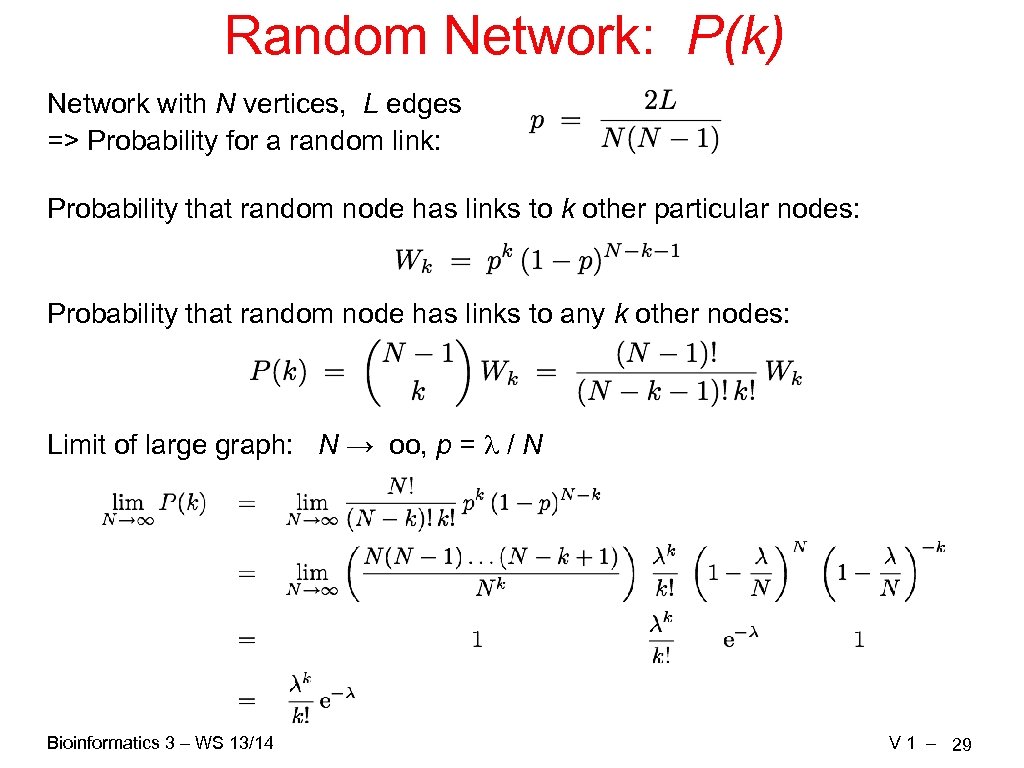Random Network: P(k) Network with N vertices, L edges => Probability for a random link: Probability that random node has links to k other particular nodes: Probability that random node has links to any k other nodes: Limit of large graph: N → oo, p = / N Bioinformatics 3 – WS 13/14 V 1 – 29

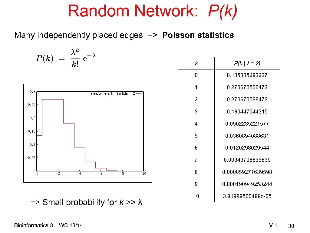Random Network: P(k) Many independently placed edges => Poisson statistics k 0 0. 270670566473 2 0. 270670566473 3 0. 180447044315 4 0. 0902235221577 5 0. 0360894088631 6 0. 0120298029544 7 0. 00343708655839 8 0. 000859271639598 9 Bioinformatics 3 – WS 13/14 0. 135335283237 1 => Small probability for k >> λ P(k | λ = 2) 0. 000190949253244 10 3. 81898506488 e-05 V 1 – 30

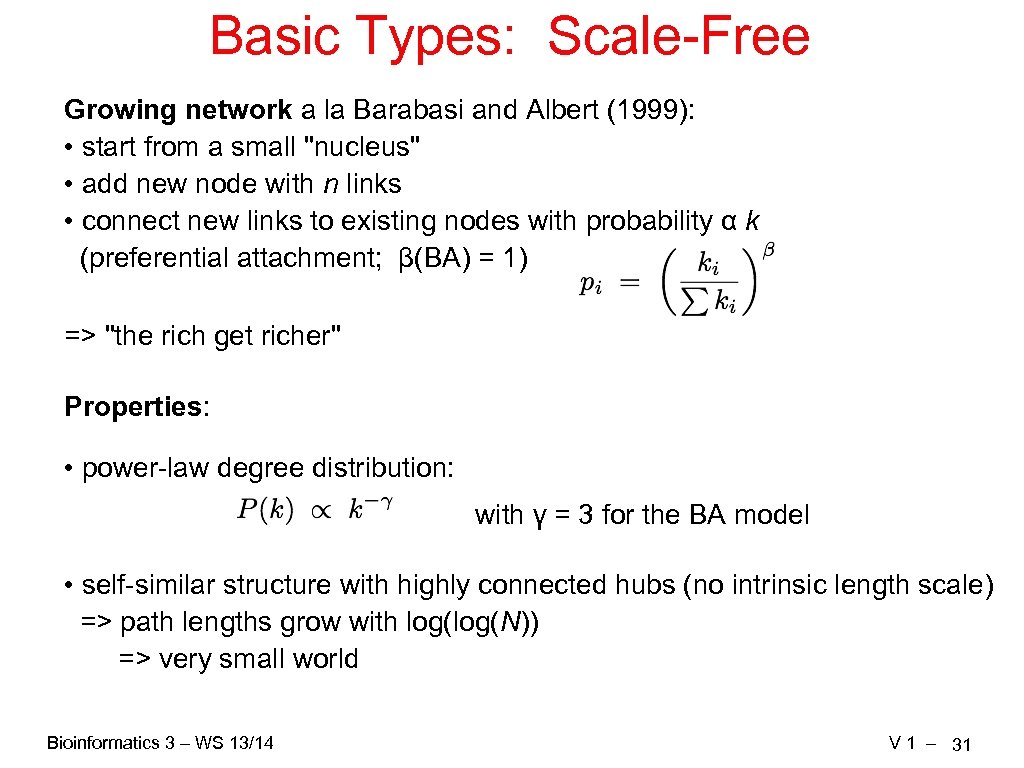Basic Types: Scale-Free Growing network a la Barabasi and Albert (1999): • start from a small "nucleus" • add new node with n links • connect new links to existing nodes with probability α k (preferential attachment; β(BA) = 1) => "the rich get richer" Properties: • power-law degree distribution: with γ = 3 for the BA model • self-similar structure with highly connected hubs (no intrinsic length scale) => path lengths grow with log(N)) => very small world Bioinformatics 3 – WS 13/14 V 1 – 31

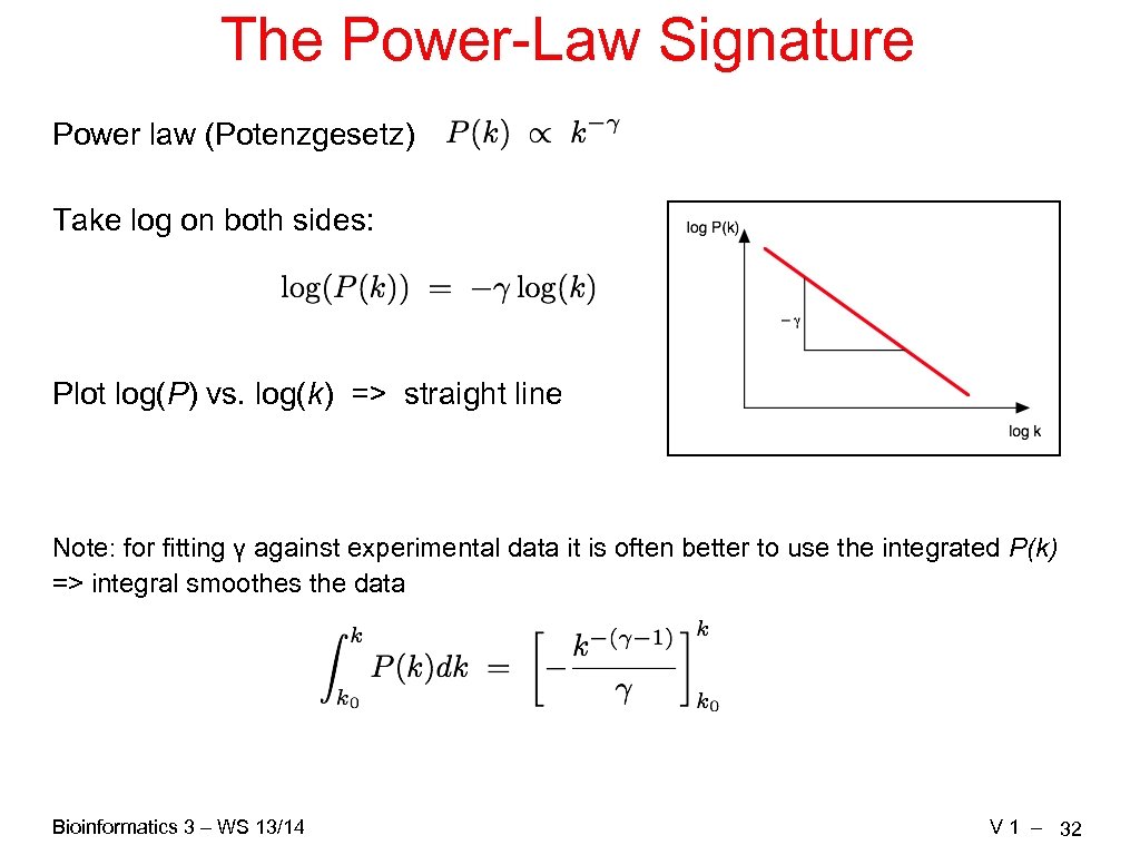The Power-Law Signature Power law (Potenzgesetz) Take log on both sides: Plot log(P) vs. log(k) => straight line Note: for fitting γ against experimental data it is often better to use the integrated P(k) => integral smoothes the data Bioinformatics 3 – WS 13/14 V 1 – 32

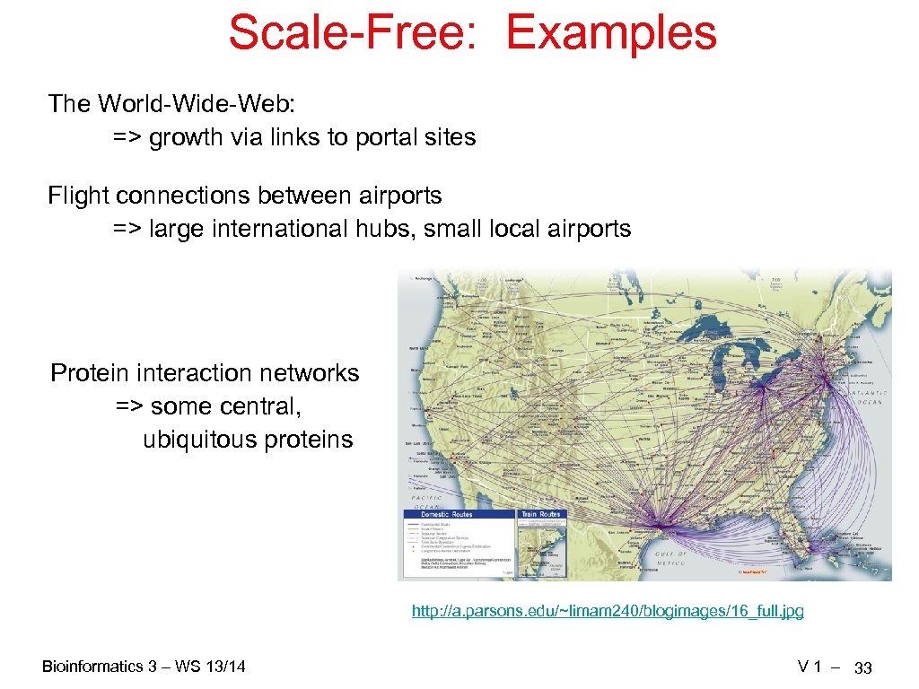Scale-Free: Examples The World-Wide-Web: => growth via links to portal sites Flight connections between airports => large international hubs, small local airports Protein interaction networks => some central, ubiquitous proteins http: //a. parsons. edu/~limam 240/blogimages/16_full. jpg Bioinformatics 3 – WS 13/14 V 1 – 33

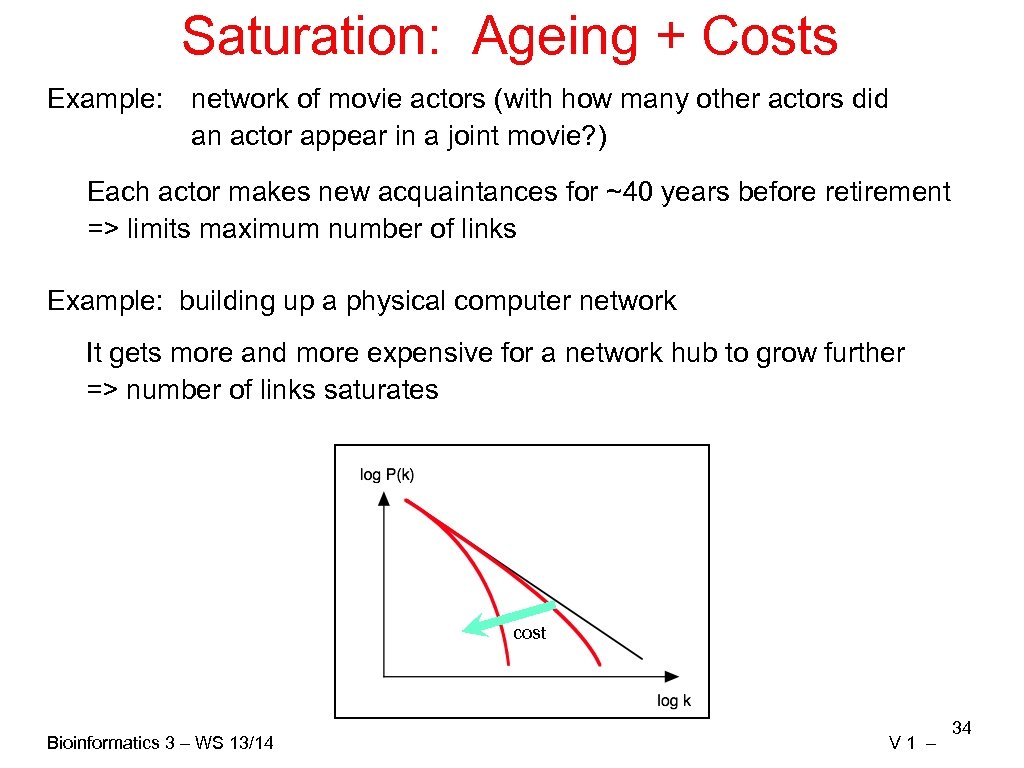Saturation: Ageing + Costs Example: network of movie actors (with how many other actors did an actor appear in a joint movie? ) Each actor makes new acquaintances for ~40 years before retirement => limits maximum number of links Example: building up a physical computer network It gets more and more expensive for a network hub to grow further => number of links saturates cost Bioinformatics 3 – WS 13/14 V 1 – 34

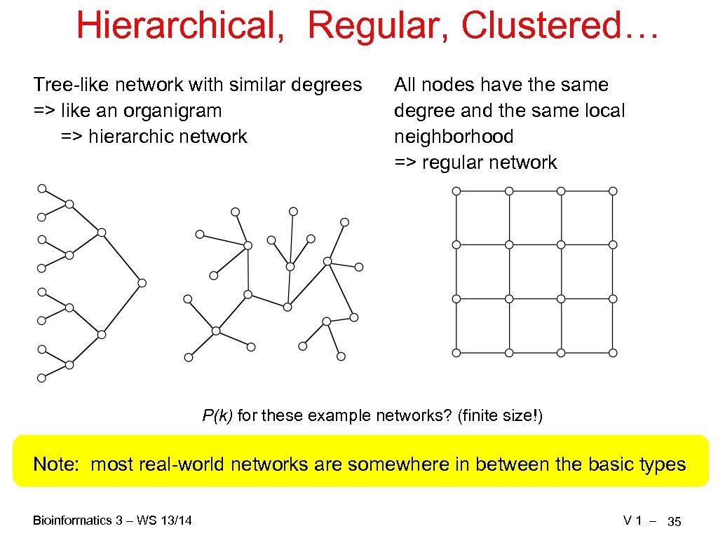Hierarchical, Regular, Clustered… Tree-like network with similar degrees => like an organigram => hierarchic network All nodes have the same degree and the same local neighborhood => regular network P(k) for these example networks? (finite size!) Note: most real-world networks are somewhere in between the basic types Bioinformatics 3 – WS 13/14 V 1 – 35

Summary What you learned today: => networks are everywhere => how to get the "Schein" for BI 3 => basic network types and definitions: random, scale-free, degree distribution, Poisson distribution, ageing, … Next lecture: => clusters, percolation => algorithm on a graph: Dijkstra's shortest path algorithm => looking at graphs: graph layout Further Reading: R. Albert and A–L Barabási, „Statistical mechanics of complex networks“ Rev. Mod. Phys. 74 (2002) 47 -97 Bioinformatics 3 – WS 13/14 V 1 – 36