Using Statistical Methods for Environmental Science and Management

Using Statistical Methods for Environmental Science and Management Graham Mc. Bride, NIWA, Hamilton g. mcbride@niwa. co. nz Statistics Teachers’ Day, 25 November 2008 What do statisticians really do?

THE ROLE OF STATISTICAL METHODS: MY VIEW • Separate randomness from pattern • Make inferences about the world, based on data from samples • Help to design sampling programmes (use resources efficiently) • Help to establish cause and effect • Can’t “prove anything with statistics”

“Three kinds of lies” Insult, or compliment? There are three kinds of lies – lies, damned lies, and statistics Who said that? – Mark Twain (1835 – 1910) “Figures often beguile me, particularly when I have the arranging of them myself” – Benjamin Disraeli (1804 – 1881) Sought to discredit true British soldier casualty figures in the Crimean War (1853 – 1856) Who came first? (Twain cites Disraeli!)

What you should do • Establish the context of your work (what do people want to know, and why do they want to know that? ) • Consult with others, e. g. , to discuss whether a proposed sampling programme can actually be done • Discuss the appropriate burden-of-proof (e. g. , drinking water standards minimise the consumer’s risk, not the producer’s risk)

What you should not do • Confuse association and causation (pp. 267 -8 of Barton, Sigma Mathematics) • Ignore other lines-of-evidence (Bradford-Hill criteria), such as – Can the cause reach the location of the effect? – Is the finding plausible? – Can you explain inconsistencies with other evidence? • Be ignorant of how statistical procedures work – The computer said so

What you should not do • Believe that there is only one “statistically correct” way of analysing data – There are lots of good ways; many more bad and wrong ways too • Not consider bias and imprecision in your data

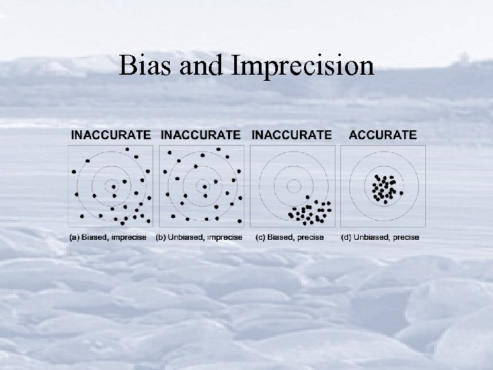Bias and Imprecision

What you might have to do • Use non-standard methods, e. g. , – non-parametric (rank) methods for highly skewed data (very common in aquatic studies) • e. g. , linear trend or monotonic trend? • Read rather widely – Statistics is not a cut-and-dried subject; there are still some fundamental debates about statistical inference, especially the Bayesians versus the frequentists—both approaches have their place

What you also might have to do • Answer this question: “What is P” – Result of a hypothesis test – Used (over-used!) routinely, so you’ll need to know • P = Prob(data at least as extreme if the tested hypothesis is true) • Not the probability of the truth of the hypothesis • Relate results to confidence intervals

EXAMPLE Increasing pressure on freshwaters Is there evidence of associated deterioration (or improvements) in rivers?

600000 4 Cows 3 400000 2. 5 300000 2 1. 5 200000 1 100000 Data source: 1 Fertilizer consumption – UN Food & Agriculture Organisation 2 Cows –Livestock Improvement NZ Dairy Statistics 2003 2002 2001 2000 1999 1998 1997 1996 1995 1994 1993 1992 1991 1990 1989 0 0. 5 0 Cow numbers (millions) 2 3. 5 Total Phosphorus 500000 1988 Fertilizer consumption (tonnes) 1 Total Nitrogen

A National River Water Quality Network for New Zealand (1989) GOAL To provide scientifically defensible information on the important physical, chemical, and biological characteristics of a selection of the nation’s rivers as a basis for advising the Minister of Science and other Ministers of the Crown of the trends and status of these waters OBJECTIVES 1. Detect significant trends in water quality 2. Develop better understanding of water resources, and hence to better assist their management

NRWQN structure • 77 sites on 35 rivers • All sites have reliable flow data • Sites are sampled by regional Field Teams • 14 WQ parameters (monthly) • Data available (search for WQIS www. niwa. co. nz

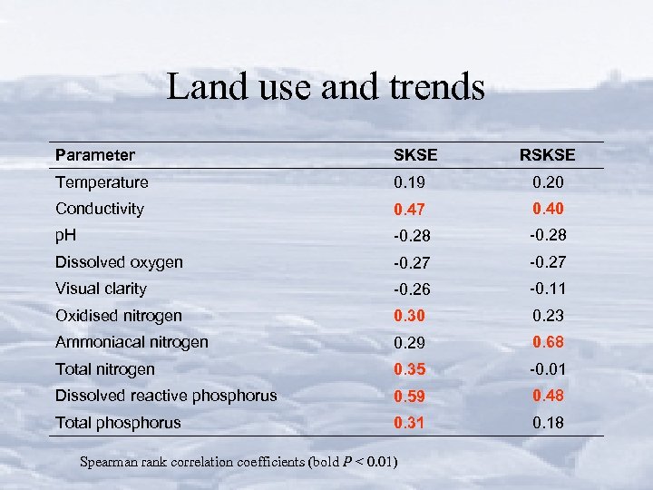
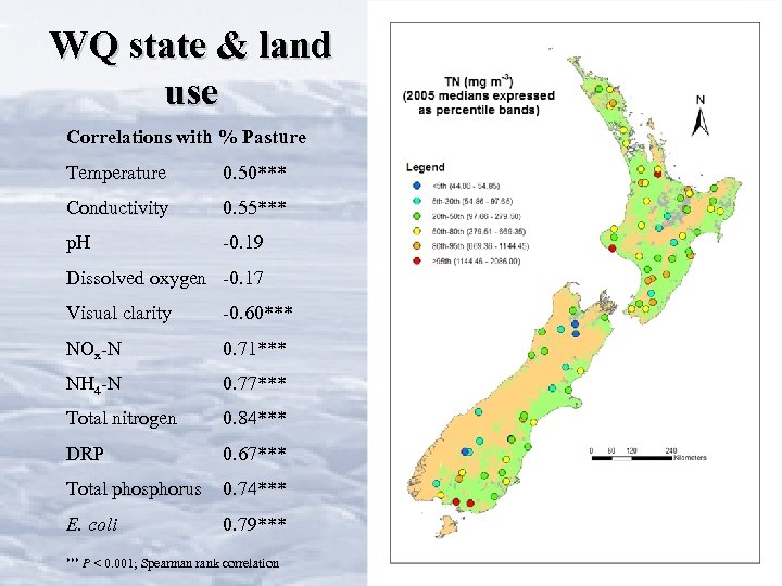WQ state & land use Correlations with % Pasture Temperature 0. 50*** Conductivity 0. 55*** p. H -0. 19 Dissolved oxygen -0. 17 Visual clarity -0. 60*** NOx-N 0. 71*** NH 4 -N 0. 77*** Total nitrogen 0. 84*** DRP 0. 67*** Total phosphorus 0. 74*** E. coli 0. 79*** P < 0. 001; Spearman rank correlation

WQ Trends 1989 -2005 • Calculated annual medians from monthly data at each site for each parameter • Took the 77 datapoints for each year and calculated the 5 th, 50 th, and 95 th percentile values • The 50 th percentile gives us a picture of what is happening in a national “average” river in terms of annual median water quality data • The 5 th and 95 th percentiles tell us about changes over time in our “best” and “worst” rivers. • Trends in these values were assessed using the Spearman rank correlation coefficient (r. S).

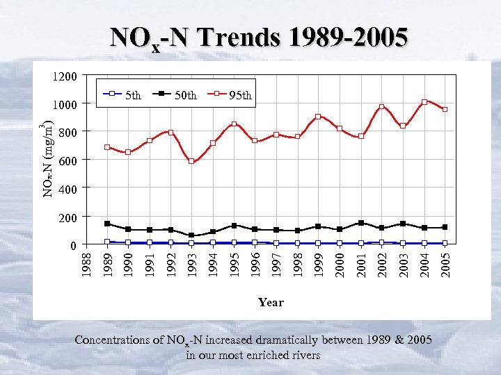NOx-N Trends 1989 -2005 1200 5 th 95 th 800 600 400 Year Concentrations of NOx-N increased dramatically between 1989 & 2005 in our most enriched rivers 2005 2004 2003 2002 2001 2000 1999 1998 1997 1996 1995 1994 1992 1991 1990 1989 0 1993 200 1988 3 NOx-N (mg/m ) 1000 50 th

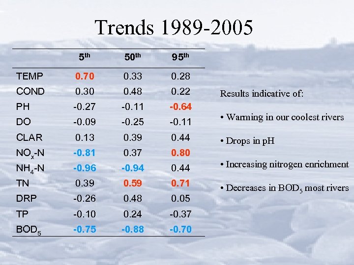Trends 1989 -2005 5 th 50 th 95 th TEMP 0. 70 0. 33 0. 28 COND 0. 30 0. 48 0. 22 PH -0. 27 -0. 11 -0. 64 DO -0. 09 -0. 25 -0. 11 CLAR 0. 13 0. 39 0. 44 NOx-N -0. 81 0. 37 0. 80 NH 4 -N -0. 96 -0. 94 0. 44 • Increasing nitrogen enrichment TN 0. 39 0. 59 0. 71 DRP -0. 26 0. 48 0. 05 • Decreases in BOD 5 most rivers TP -0. 10 0. 24 -0. 37 BOD 5 -0. 75 -0. 88 -0. 70 Results indicative of: • Warming in our coolest rivers • Drops in p. H

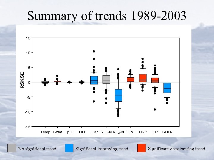
Trends 1989 -2003 • More formal analysis of trends carried out on monthly data (1989 -2003) at all 77 sites • Seasonal Kendall test • Data were flow-adjusted using LOWESS (many WQ parameters can be strongly influenced by discharge) • Used a binomial test to indicate a “national trend” • Discriminate between “significant” (i. e. P < 0. 05) and “meaningful” trends (i. e. , P < 0. 05 and slope > 1% of median value per annum).

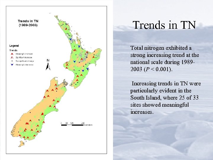Trends in TN Total nitrogen exhibited a strong increasing trend at the national scale during 19892003 (P < 0. 001). Increasing trends in TN were particularly evident in the South Island, where 25 of 33 sites showed meaningful increases.

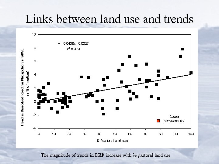
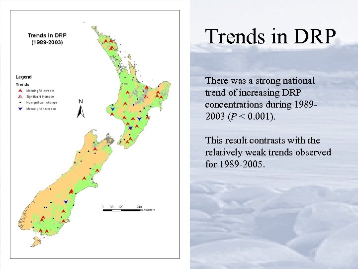Trends in DRP There was a strong national trend of increasing DRP concentrations during 19892003 (P < 0. 001). This result contrasts with the relatively weak trends observed for 1989 -2005.

Summary of trends 1989 -2003 15 10 RSKSE 5 Plot 1 0 -5 -10 -15 Temp Cond No significant trend p. H DO Clar NOx-N NH 4 -N TN Significant improving trend DRP TP BOD 5 Significant deteriorating trend

Links between land use and trends 10 Trend in Dissolved Reactive Phospohorus (SKSE as % of median) y = 0. 0406 x - 0. 0027 8 R 2 = 0. 31 6 4 2 0 -2 Lower Manawatu Rv. -4 0 10 20 30 40 50 60 70 80 % Pastoral land use The magnitude of trends in DRP increase with % pastoral land use 90 100

Land use and trends Parameter SKSE Temperature 0. 19 0. 20 Conductivity 0. 47 0. 40 p. H -0. 28 Dissolved oxygen -0. 27 Visual clarity -0. 26 -0. 11 Oxidised nitrogen 0. 30 0. 23 Ammoniacal nitrogen 0. 29 0. 68 Total nitrogen 0. 35 -0. 01 Dissolved reactive phosphorus 0. 59 0. 48 Total phosphorus 0. 31 0. 18 Spearman rank correlation coefficients (bold P < 0. 01) RSKSE

Conclusions • Strong associations between nutrient concentrations and %pastoral land cover at the national scale (State) • Rivers draining large areas of pastoral land have deteriorated significantly over the last 17 years with respect to nitrogen concentrations (Trends) • The magnitude of trends in some parameters is associated with extent of pastoral land use • Decreasing trends in NH 4 -N and BOD 5 indicative of improvements in point source management • Increasing trends in nutrients indicative of increasing pressure from agriculture

EXAMPLE: Water quality-human health risk assessment, quantitative approach Christchurch City Wastewater Outfall

Quantitative Microbial Health Risk Assessment (QMHRA) • Identify hazards (pathogens) • Quantify exposure (swimming, shellfish consumption) • Assess dose-response • Characterise risk

Hazard vs. Risk • Hazards can cause harm, after exposure • Risk cannot occur if no exposure • Can have hazard without risk • But not vice versa!

Christchurch hazards—viruses only From an extensive list (next slide): • Swimming – adenovirus (respiratory) – rotavirus – enterovirus (Echovirus 12) • Shellfish consumption (raw) – enteroviruses – rotavirus – hepatitis A

Dose-response curves

Accounting for variability and uncertainty • Exposure is variable – e. g. , individuals’ swim duration • Dose-response is uncertain – only some pathogen strains in clinical trials – trials limited to healthy adults • Describe using statistical distributions in a Monte Carlo analysis

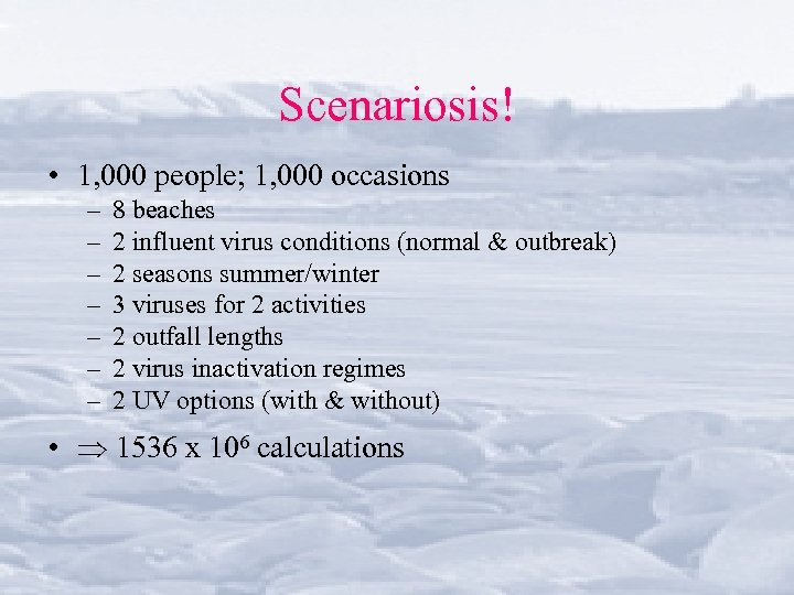Scenariosis! • 1, 000 people; 1, 000 occasions – – – – 8 beaches 2 influent virus conditions (normal & outbreak) 2 seasons summer/winter 3 viruses for 2 activities 2 outfall lengths 2 virus inactivation regimes 2 UV options (with & without) • 1536 x 106 calculations

Calculation sequence

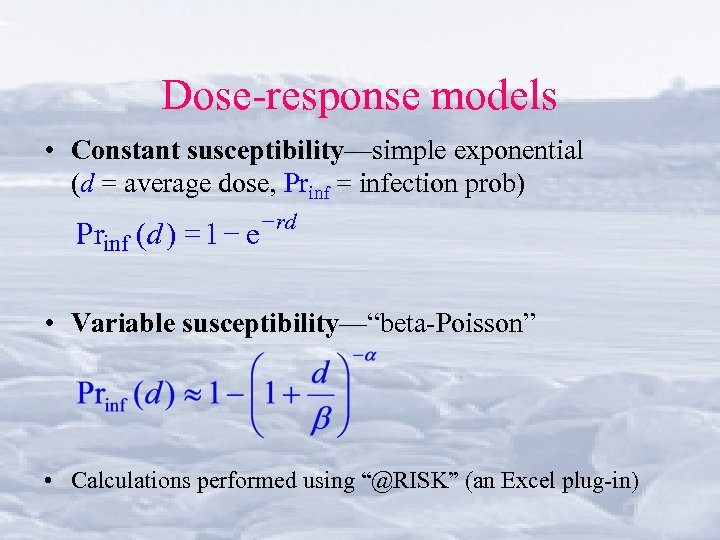Dose-response models • Constant susceptibility—simple exponential (d = average dose, Prinf = infection prob) Prinf ( d ) = 1 - e - rd • Variable susceptibility—“beta-Poisson” • Calculations performed using “@RISK” (an Excel plug-in)

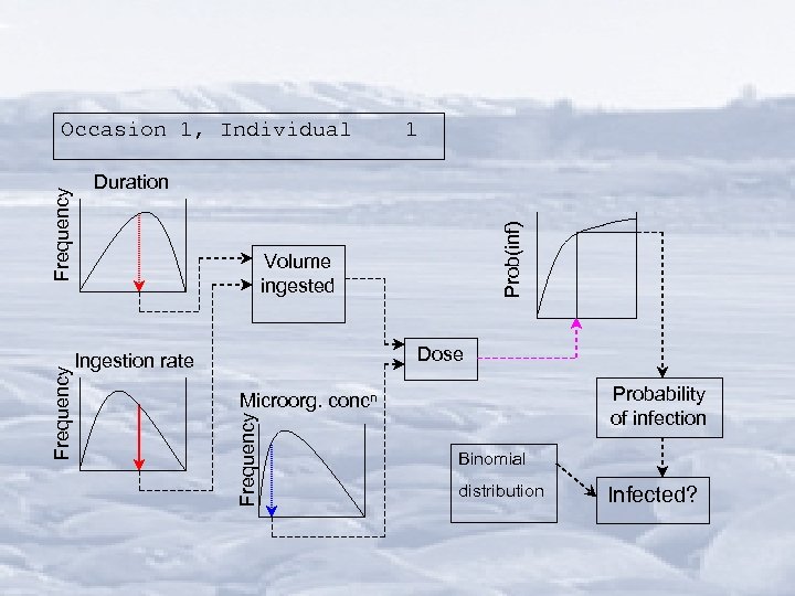1 Prob(inf) Duration Volume ingested Dose Ingestion rate Probability of infection Microorg. concn Frequency Occasion 1, Individual Binomial distribution Infected?

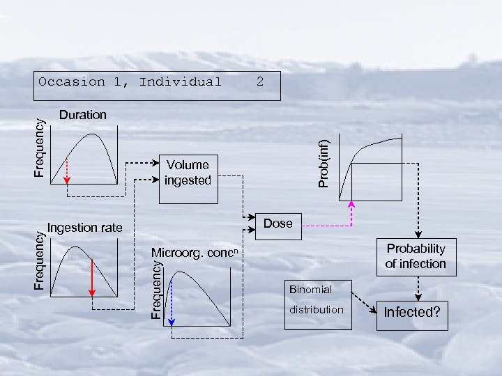2 Prob(inf) Duration Volume ingested Dose Ingestion rate Probability of infection Microorg. concn Frequency Occasion 1, Individual Binomial distribution Infected?

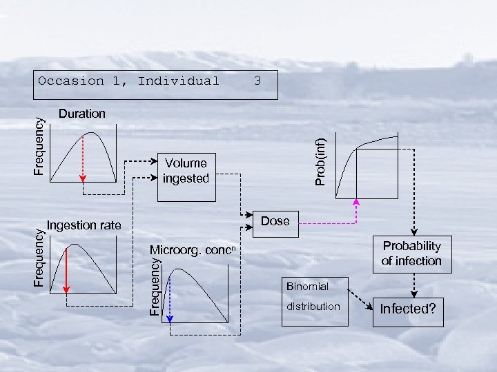3 Prob(inf) Duration Volume ingested Dose Ingestion rate Probability of infection Microorg. concn Frequency Occasion 1, Individual Binomial distribution Infected?

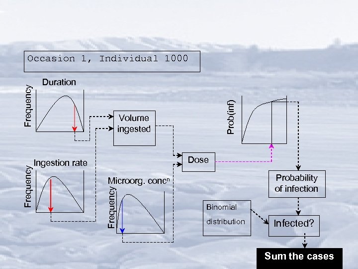Prob(inf) Duration Volume ingested Dose Ingestion rate Probability of infection Microorg. concn Frequency Occasion 1, Individual 1000 Binomial distribution Infected? Sum the cases

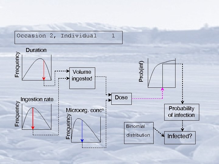1 Prob(inf) Duration Volume ingested Dose Ingestion rate Probability of infection Microorg. concn Frequency Occasion 2, Individual Binomial distribution Infected?

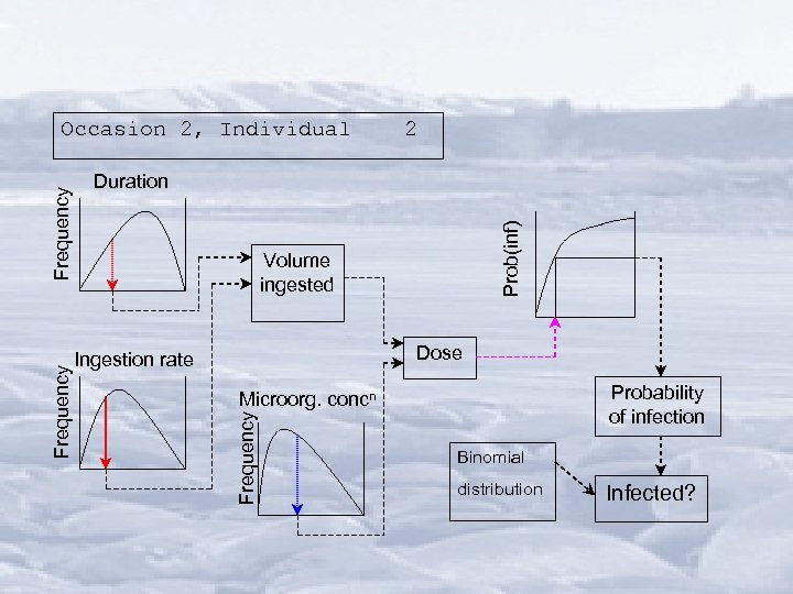2 Prob(inf) Duration Volume ingested Dose Ingestion rate Probability of infection Microorg. concn Frequency Occasion 2, Individual Binomial distribution Infected?

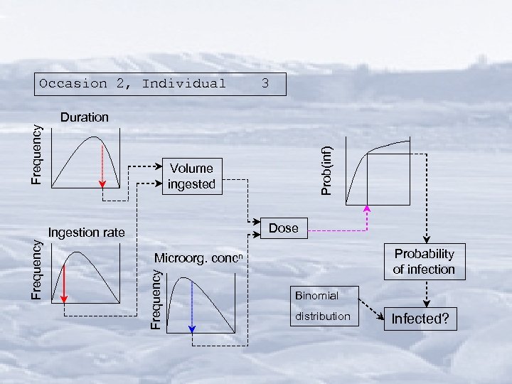Occasion 2, Individual 3 Volume ingested Dose Ingestion rate Probability of infection Microorg. concn Frequency Prob(inf) Frequency Duration Binomial distribution Infected?

Characterising the results • Risk percentiles—percent of time the risk is below a stated value • IIR—Individual Infection Risk (total number of calculated infections divided by total number of exposures)

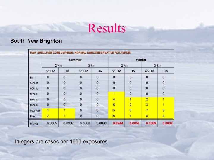Results South New Brighton Integers are cases per 1000 exposures

IIR: Normal influent, South Brighton adenovirus, swim Numbers are percentages. Mf. E/Mo. H (2003) guidelines: <0. 3% = “Very good”.

IIR: Normal influent, South Brighton rotavirus, shellfish Numbers are percentages.

IIR: Outbreak influent, South Brighton adenovirus, swim Numbers are percentages. Mf. E/Mo. H (2003) guidelines: 1. 9 - 3. 9% = “Fair” - “Poor”.

IIR: Outbreak influent, South Brighton rotavirus, shellfish Numbers are percentages.

IIR: Outbreak influent, South Brighton hepatitis A, shellfish Numbers are percentages.

Statistical modelling can reveal important information gaps • • Bioaccumulation factors for NZ shellfish Dose-response for norovirus (new study published) Detailed exposure data (ingestion rates etc. ) Constancy of virulence? Campylobacter in shellfish? Better methods for uncertainty analysis Better models for illness, cf. infection

Conclusions • Longer outfall no UV still has higher risk than shorter outfall with UV • But risks low • What if UV doesn’t work 24/7 (technology breakdown, power outage, …) • Decision: longer outfall, no UV

Semi-Quantitative approach Use when hazards and exposures are less well-defined and more widespread Paradigm is: Risk score = Likelihood x Consequences Use scores as a relative measure of risk. Use panel of “experts”; may solicit list of hazards from affected community

Hazards • • Pathogens (from humans and animals) Chemicals Algal toxins Physical objects

“End-points” (exposures) • • Recreational contact Drinking water consumption Consumptions of aquatic organisms Food? (more difficult)

The delivery chain • Can be called “hazardous event” • How does the hazard get from its origin to the point of exposure?

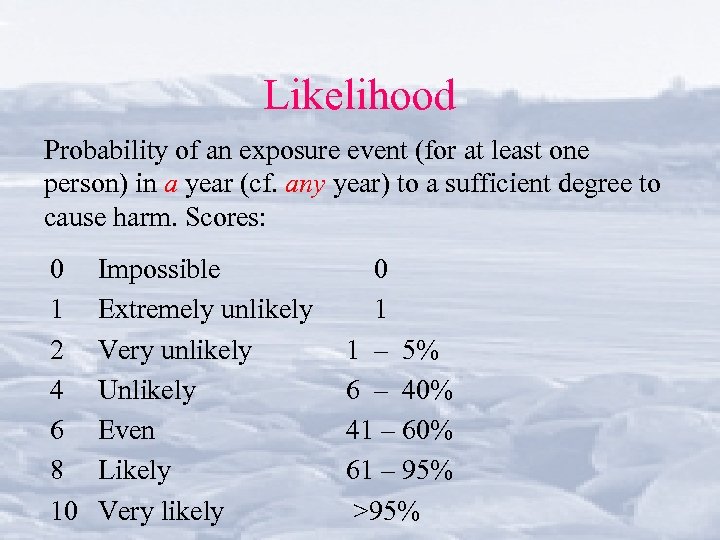Likelihood Probability of an exposure event (for at least one person) in a year (cf. any year) to a sufficient degree to cause harm. Scores: 0 1 2 4 6 8 10 Impossible Extremely unlikely Very unlikely Unlikely Even Likely Very likely 0 1 1 – 5% 6 – 40% 41 – 60% 61 – 95% >95%

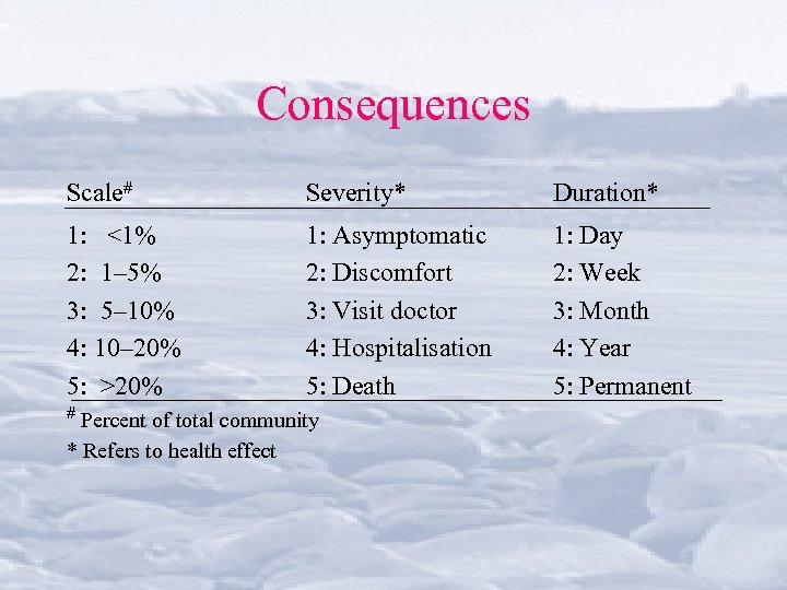Consequences Scale# Severity* Duration* 1: <1% 2: 1– 5% 3: 5– 10% 4: 10– 20% 5: >20% 1: Asymptomatic 2: Discomfort 3: Visit doctor 4: Hospitalisation 5: Death 1: Day 2: Week 3: Month 4: Year 5: Permanent # Percent of total community * Refers to health effect

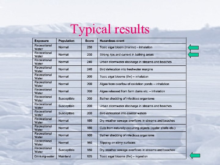Typical results

Conclusions • Use QRA for well-defined “local” problems • Use semi-quantitative methods for broader-scale problems • Risk assessment identifies many knowledge gaps, some need urgent attention • Most difficult gap often the “delivery chain” • Can update assessments with new data • Especially useful in ranking risks

EXAMPLE Compliance with Drinking Water Standards How to assess compliance with microbial limits? • Can’t sample everything • Need high assurance that supply isn’t contaminated in some assessment period; can’t be fully assured • Mo. H then said: “We want to be 95% confident that the water is uncontaminated for 95% of the time. What should the compliance rule be? ”

What kind of a question is this? • Bayesian – It asks about the probability of an hypothesis, given data that we will collect – Frequentist (“classical” methods) ask about the probability of data assuming an hypothesis to be true • Precautionary (not “permissive”) – Benefit of doubt goes to the consumer, not to the supplier • One-sided – Hypothesis to be tested is breach, not compliance

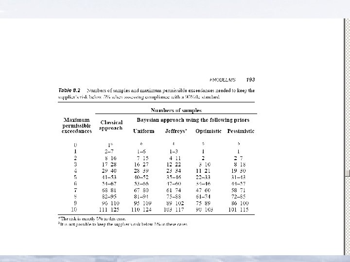Results

Results

Policy Implications • Results in Table 8. 2 now incorporated into 2005 Drinking-water Standards for New Zealand – http: //www. moh. govt. nz/moh. nsf/0/12 F 2 D 7 FFADC 900 A 4 CC 256 FAF 0007 E 8 A 0/$File/drinkingwaterstandardsnz-2005. pdf

EXAMPLE Effect of microbial contamination on swimmers’ health Epidemiological study at 7 NZ beaches

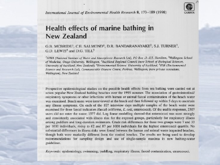
Main Findings • Using generalized regression models – Evidence of respiratory illness effects related to microbial contamination – Human- and animal-waste impacted beaches not separable in terms of health effects – Both were separable from “control” beaches

Policy implications • Human and animal wastes no longer distinguished in terms of health risks • Result incorporated into new guidelines – http: //www. mfe. govt. nz/publications/water/microbiological-quality-jun 03/