Using and Building Comprehensive GCMs Paul J Kushner

Using and Building Comprehensive GCMs Paul J. Kushner University of Toronto GCC Summer School Banff 2005

Outline • Review • The Model Development Trajectory • Pitfalls of Using GCMs • Building a comprehensive GCM: GFDL AM 2 • Conclusion

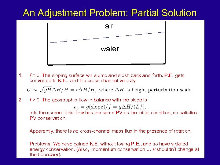
An Adjustment Problem: Partial Solution air water 1. f = 0. The sloping surface will slump and slosh back and forth. P. E. gets converted to K. E. , and the cross-channel velocity 2. f > 0. The geostrophic flow in balance with the slope is into the screen. This flow has the same PV as the initial condition, so satisfies PV conservation. Apparently, there is no cross-channel mass flux in the presence of rotation. Problems: We have gained K. E. without losing P. E. , and so have violated energy conservation. (Also, momentum conservation … v shouldn’t change at the boundary).

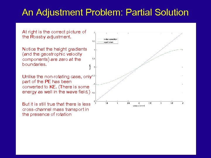
An Adjustment Problem: Partial Solution At right is the correct picture of the Rossby adjustment. Notice that the height gradients (and the geostrophic velocity components) are zero at the boundaries. Unlike the non-rotating case, only part of the PE has been converted to KE. (There is some energy as well in the wave field. ) But it is still true that there is less cross-channel mass transport in the presence of rotation

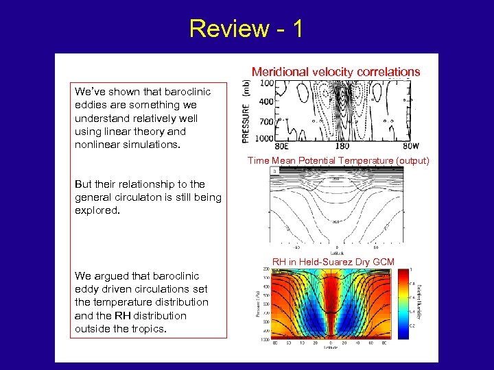
Review - 1 Meridional velocity correlations We’ve shown that baroclinic eddies are something we understand relatively well using linear theory and nonlinear simulations. Time Mean Potential Temperature (output) But their relationship to the general circulaton is still being explored. Hartmann 1994 RH in Held-Suarez Dry GCM We argued that baroclinic eddy driven circulations set the temperature distribution and the RH distribution outside the tropics.

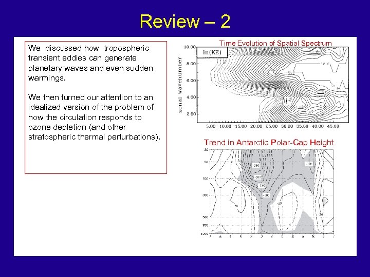
Review – 2 We discussed how tropospheric transient eddies can generate planetary waves and even sudden warmings. We then turned our attention to an idealized version of the problem of how the circulation responds to ozone depletion (and other stratospheric thermal perturbations). Time Evolution of Spatial Spectrum Trend in Antarctic Polar-Cap Height

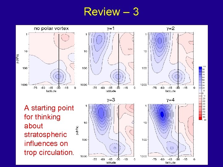
Review – 3 A starting point for thinking about stratospheric influences on trop circulation.

Moving On • We finished by pointing out the strengths and weaknesses of the simple models … and decided it was time to move on to GCMs. • I will start with examples of potential pitfalls of GCMbased research (not to be critical … but to help you avoid them). • Then, a more upbeat story … personal experiences of model development at GFDL.

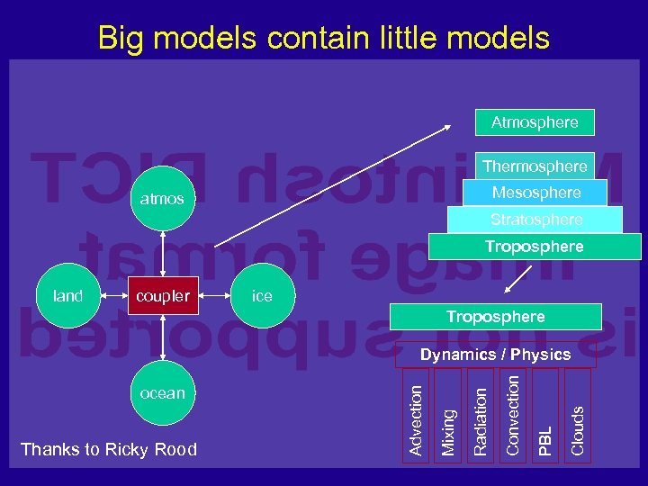
Big models contain little models Atmosphere Thermosphere Mesosphere atmos Stratosphere Troposphere land coupler ice Troposphere Clouds PBL Convection Radiation Thanks to Ricky Rood Mixing ocean Advection Dynamics / Physics

Big models contain little models • Each model component is associated with multiple parameters that are varied. • Approaches exist (Charles Jackson, Houtekamer (? ), others … ) to automatically estimate the best parameters to obtain some desired climate model. These are not commonly used yet. • In practice, each model component is associated with individual people who bring independent scientific judgement on development.

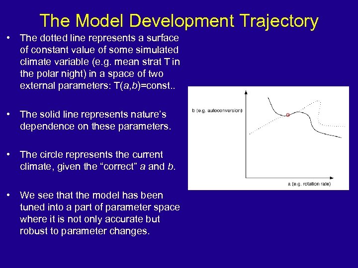
The Model Development Trajectory • The dotted line represents a surface of constant value of some simulated climate variable (e. g. mean strat T in the polar night) in a space of two external parameters: T(a, b)=const. . • The solid line represents nature’s dependence on these parameters. • The circle represents the current climate, given the “correct” a and b. • We see that the model has been tuned into a part of parameter space where it is not only accurate but robust to parameter changes.

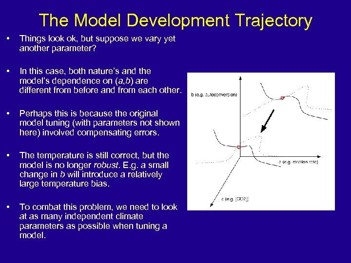
The Model Development Trajectory • Things look ok, but suppose we vary yet another parameter? • In this case, both nature’s and the model’s dependence on (a, b) are different from before and from each other. • Perhaps this is because the original model tuning (with parameters not shown here) involved compensating errors. • The temperature is still correct, but the model is no longer robust. E. g. a small change in b will introduce a relatively large temperature bias. • To combat this problem, we need to look at as many independent climate parameters as possible when tuning a model.

Pitfalls of Using GCMs

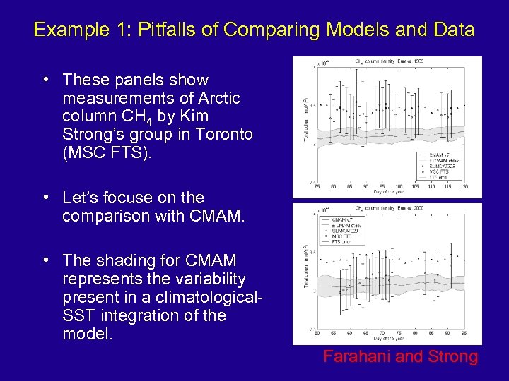
Example 1: Pitfalls of Comparing Models and Data • These panels show measurements of Arctic column CH 4 by Kim Strong’s group in Toronto (MSC FTS). • Let’s focuse on the comparison with CMAM. • The shading for CMAM represents the variability present in a climatological. SST integration of the model. Farahani and Strong

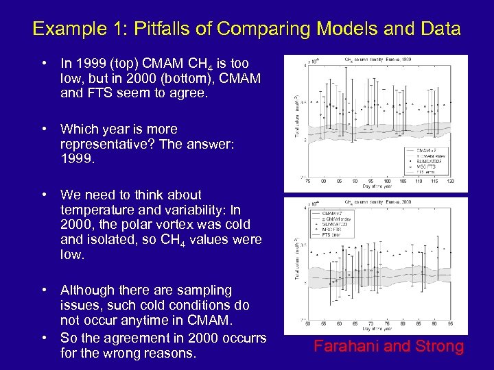
Example 1: Pitfalls of Comparing Models and Data • In 1999 (top) CMAM CH 4 is too low, but in 2000 (bottom), CMAM and FTS seem to agree. • Which year is more representative? The answer: 1999. • We need to think about temperature and variability: In 2000, the polar vortex was cold and isolated, so CH 4 values were low. • Although there are sampling issues, such cold conditions do not occur anytime in CMAM. • So the agreement in 2000 occurrs for the wrong reasons. Farahani and Strong

Example 2: Non-Robustness • A model intercomparison of climate sensitivity. • Soden et al. compare two rapidly developing models (GFDL/AM 2 and NCAR/CAM 2) initially and then a year later. • No observed data is involved, and no (explicit) coordination between the models occurs.

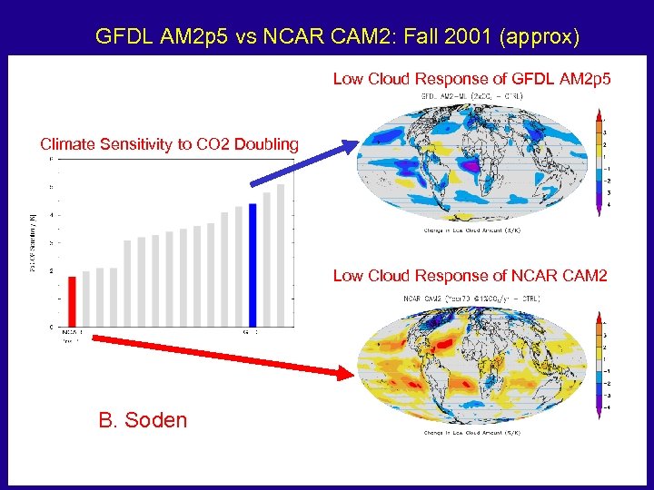
GFDL AM 2 p 5 vs NCAR CAM 2: Fall 2001 (approx) Low Cloud Response of GFDL AM 2 p 5 Climate Sensitivity to CO 2 Doubling Low Cloud Response of NCAR CAM 2 B. Soden

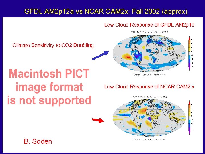
GFDL AM 2 p 12 a vs NCAR CAM 2 x: Fall 2002 (approx) Low Cloud Response of GFDL AM 2 p 10 Climate Sensitivity to CO 2 Doubling Low Cloud Response of NCAR CAM 2. x B. Soden

Example 2: More Non-Robustness • With Sigmond, Scinocca, and Held, we have been looking at the robustness of the circulation response to climate change. • We systematically vary resolution and look at its impact. • Many features (e. g. tropical temperatures) respond robustly. We won’t focus on those!

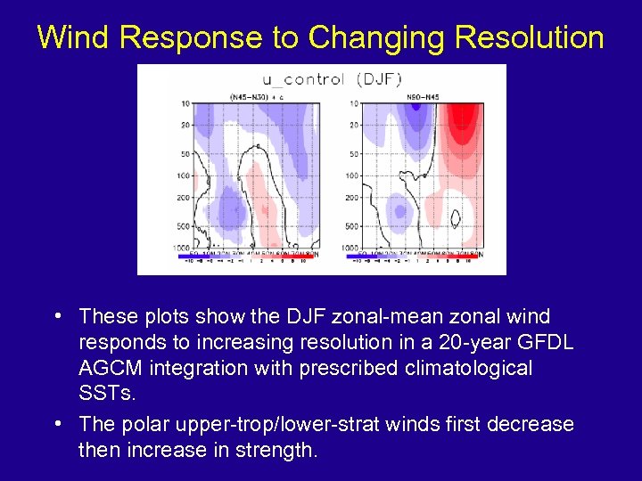
Wind Response to Changing Resolution • These plots show the DJF zonal-mean zonal wind responds to increasing resolution in a 20 -year GFDL AGCM integration with prescribed climatological SSTs. • The polar upper-trop/lower-strat winds first decrease then increase in strength.

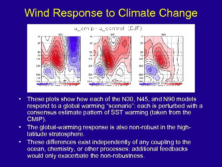
Wind Response to Climate Change • These plots show each of the N 30, N 45, and N 90 models respond to a global warming “scenario”: each is perturbed with a consensus estimate pattern of SST warming (taken from the CMIP). • The global-warming response is also non-robust in the highlatitude stratosphere. • These differences exist independently of any coupling to the ocean, chemistry, or other processes: additional feedbacks would only exacerbate the non-robustness.

Enough Pitfalls! … • … Let’s move on to a cheerier topic. • How GCM development should work: 0. Motivation: Decide what you’re after. 1. Building: choosing pieces, putting them together. 2. Implementation and tuning: a systematic cycle of hypothesis testing, diagnosis, modification. • How it really works: ß A rather freewheeling and messy exercise.

Building a comprehensive GCM: GFDL AM 2

GFDL Model Development (2000 – Present) • By mid-1990’s, GFDL had several climate models maintained by different scientific groups across the lab. • Although much groundbreaking research had been done with them, the models were generally out of date, and development efforts subcritical. • The advent of parallel computer architectures forced the lab to think about how to best develop the lab’s modeling capabilities

Important Decisions 1. To develop a “workhorse” coupled oceanatmosphere model that would serve climate and seasonal-prediction needs. The aims of this coupled model: ß To run without flux adjustments. ß To simulate a reasonable climatological SST distribution, ENSO, and thermohaline circulation. ß To be able to run about 4 100 -y simulations per month using less than half the lab’s available CPU hours.

Important Decisions 2. To organize the effort around teams devoted to each model component (atmosphere, ocean, etc. ) instead of science projects. 3. To improve the technical foundation of development (FMS, automated diagnostic tools).

GAMDT • “Global Atmospheric Model Development Team” charged with creation of an atmosphere/land “trunk” component (AM 2/LM 2) of GFDL’s next-generation Earth-systems model (CM 2) • At the same time, to pursue atmospheric model development in new areas (higher resolution, stratosphere, aerosol transport & chemistry, land/biosphere…)

GAMDT Organization • Members from four scientific & technical groups at GFDL. • Experts work with their own components. • Weekly meetings focusing on diagnostics and progress.

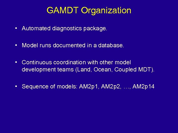
GAMDT Organization • Automated diagnostics package. • Model runs documented in a database. • Continuous coordination with other model development teams (Land, Ocean, Coupled MDT). • Sequence of models: AM 2 p 1, AM 2 p 2, …, AM 2 p 14

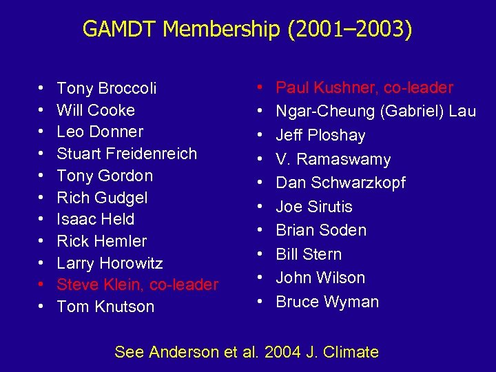
GAMDT Membership (2001– 2003) • • • Tony Broccoli Will Cooke Leo Donner Stuart Freidenreich Tony Gordon Rich Gudgel Isaac Held Rick Hemler Larry Horowitz Steve Klein, co-leader Tom Knutson • • • Paul Kushner, co-leader Ngar-Cheung (Gabriel) Lau Jeff Ploshay V. Ramaswamy Dan Schwarzkopf Joe Sirutis Brian Soden Bill Stern John Wilson Bruce Wyman See Anderson et al. 2004 J. Climate

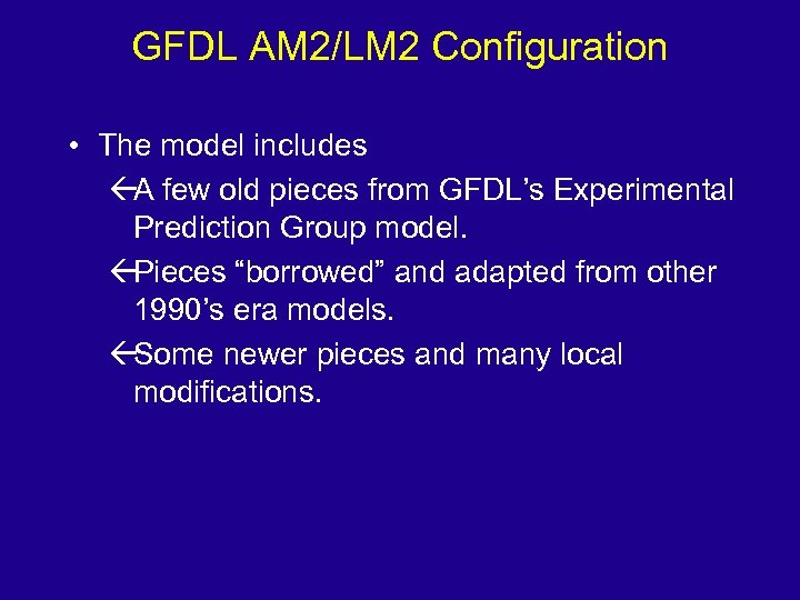
GFDL AM 2/LM 2 Configuration • The model includes ßA few old pieces from GFDL’s Experimental Prediction Group model. ßPieces “borrowed” and adapted from other 1990’s era models. ßSome newer pieces and many local modifications.

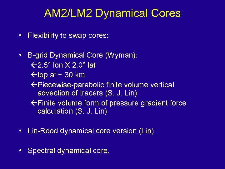
AM 2/LM 2 Dynamical Cores • Flexibility to swap cores: • B-grid Dynamical Core (Wyman): ß 2. 5° lon X 2. 0° lat ßtop at ~ 30 km ßPiecewise-parabolic finite volume vertical advection of tracers (S. J. Lin) ßFinite volume form of pressure gradient force calculation (S. J. Lin) • Lin-Rood dynamical core version (Lin) • Spectral dynamical core.

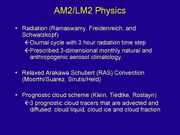
AM 2/LM 2 Physics • Radiation (Ramaswamy, Freidenreich, and Schwarzkopf) ßDiurnal cycle with 3 hour radiation time step ßPrescribed 3 -dimensional monthly natural and anthropogenic aerosol climatology. • Relaxed Arakawa Schubert (RAS) Convection (Moorthi/Suarez, Sirutis/Held) • Prognostic cloud scheme (Klein, Tiedtke, Rostayn) ß 3 prognostic cloud tracers that are advected and diffused: cloud liquid, cloud ice and cloud fraction

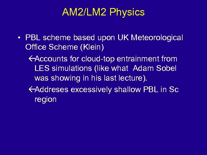
AM 2/LM 2 Physics • PBL scheme based upon UK Meteorological Office Scheme (Klein) ßAccounts for cloud-top entrainment from LES simulations (like what Adam Sobel was showing in his last lecture). ßAddreses excessively shallow PBL in Sc region

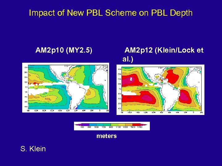
Impact of New PBL Scheme on PBL Depth AM 2 p 10 (MY 2. 5) AM 2 p 12 (Klein/Lock et al. ) meters S. Klein

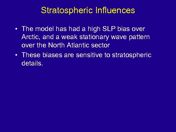
Stratospheric Influences • The model has had a high SLP bias over Arctic, and a weak stationary wave pattern over the North Atlantic sector • These biases are sensitive to stratospheric details.

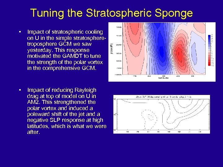
Tuning the Stratospheric Sponge • Impact of stratospheric cooling on U in the simple stratospheretroposphere GCM we saw yesterday. This response motivated the GAMDT to tune the strength of the polar vortex in the comprehensive GCM. • Impact of reducing Rayleigh drag at top of model on U in AM 2. This strengthened the polar vortex and induced a poleward shift of the jet and a negative SLP response at high latitudes, which is what we were after.

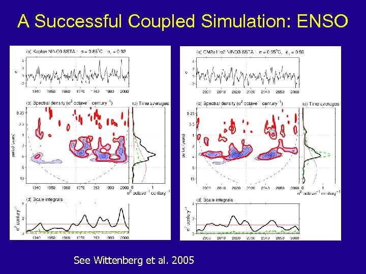
A Successful Coupled Simulation: ENSO See Wittenberg et al. 2005

Diagnostics: Model/Obs Comparisons • I will show pictures from a prescribed SST (“AMIP”) integration “AM 2 p 14. ” • These pictures, comparing model and obs, were the standard tools we used to judge the quality of a simulation (there were at least a dozen simulations in play at any given time). • We use fairly standard available datasets, each with its own strengths and weaknesses. Modellers have only a partial handle on the merits of these datasets. • The figures I will show are for AM 2 p 14 (Lin-Rood Core, Atmospheric Component of CM 2. 1) … downloaded from GFDL, please see http: //www. atmosp. physics. utoronto. ca/people/pjk/rtsfigures/ … but please don’t show without GFDL permission! • Acrobat

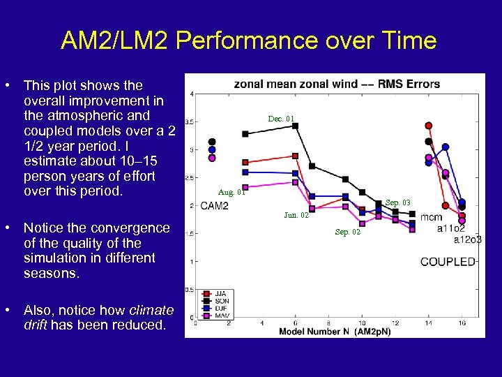
AM 2/LM 2 Performance over Time • This plot shows the overall improvement in the atmospheric and coupled models over a 2 1/2 year period. I estimate about 10– 15 person years of effort over this period. Dec. 01 Aug. 01 Sep. 03 Jun. 02 • Notice the convergence of the quality of the simulation in different seasons. • Also, notice how climate drift has been reduced. Sep. 02

Conclusions • GCMs remain the best tool for quantitative analysis of climate in the context of observations. • We have shown various pitfalls involved in using “free-running” GCMs for comparisons to observations and for climate projection. • GCM development can teach much about the climate system if we pay attention.

Conclusion • The GFDL GAMDT needed a “team” approach to build a successful model, because the models are so complicated: everyone needs to develop expertise in the model as a whole. • Software (FMS, database), organizational tools, and computer resources were also crucial. • Working on many aspects in parallel helped overcome some of the “trajectory” issues we’ve discussed.

Thanks … • … to Elham, Ricky, Michael Sigmond, Steve Klein, Isaac Held, Brian Soden, Gabriel Lau, and many others for slide material, • …. to all the participants for a great summer school, • … and to Ted for organizing it and inviting me!