Use of Expanded Input and Output Sets in

Use of Expanded Input and Output Sets in a General Parametric Cost Model Bob Fairbairn Use of Expanded Input and Output Sets in a General Parametric Cost Model 1

SSP (Subsystem Phase model) • Collection of development cost modules – General model type, with substantial logic, calibrated to data – Modules: mechanical, electronic, chip, software (COCOMO II)) • In formulation and use for several (last 12) years – Successive versions of model used on variety of projects – Including un-manned space projects (GIFTS, GLAST , MRO, SIM, assorted instruments), and manned (Transhab, SS Prop Module) – Is an ongoing development project, not static • Key distinguishing characteristics: – Developed from detailed, sub-project-level data – Uses relatively large input set, • Including number-of-instructions-type size parameters – Produces granular output for analysis: • Hours, staffing levels and dollars by function, • In discrete phases and uniform time units, • Both resource and time output at WBS level of definition Use of Expanded Input and Output Sets in a General Parametric Cost Model 2

Goals of Cost Modeling • General: – To provide as much useful information about cost and schedule as possible, in order to support project planning and to maximize return on investment • Next level: – To maximize use of available definition information – To provide detailed cost and schedule output, with many potential points of comparison for analysis – To model the process as faithfully as possible • To provide useful feedback to the modeler • To maximize understanding of model results (Constructiveness) – To make the modeling process as systematic as possible • To minimize analyst judgment in the process Use of Expanded Input and Output Sets in a General Parametric Cost Model 3

Original motivation for change: mass-based equations • In practice, observed many cases where cost should be less sensitive to weight than model results indicated • Logic, experience tell us that mass is not an ideal predictor of cost: – Mass was originally used because it was available – In the global (large-mass-range) domain, there is often a positive correlation between mass and cost, but: – In the local (small-mass-range) domain, results are inconsistent • Correlation may be insignificant (no relationship), or even negative (inverse relationship) – The need to use log-log regression to obtain a good fit should be a warning sign • Log-log r^2 is misleading • Error in original units is the relevant measure • Observed that other parameters appeared to be more related to cost than mass – Also true for fabrication costs when material cost excluded Use of Expanded Input and Output Sets in a General Parametric Cost Model 4

Supplementing mass in traditional, mass-based CERs • Introduce more variables, multivariable regressions • Some improvement (mass has a smaller effect on cost), but still many problems, e. g. : – Power function often retained as the functional form – Mass often still has a significant effect (large exponent value) • Which in turn diminishes effects of other parameters – Dependence between parameters conflicts with assumptions of independence, produces poor regression results • How frequently do analysts check for dependence between assumed independent variables? – Effects of new parameters are not modeled well by multivariable power functions and other convenient functional forms Use of Expanded Input and Output Sets in a General Parametric Cost Model 5

Supplementing mass in mass-based general models • Add relevant parameters, logic. – Get "families" of cost-to-mass curves, with complexity or scale factors (intercepts) determined by new parameters • Does not solve the mass problem – Exponent on weight, typically 0. 7 +/- 0. 2, makes its effect significant, – thereby reducing the effect of other parameters • Result: analysts have to do separate calibrations for many cost elements – Much more than would be necessary if equations were modeling the process well – Effectively reduces “general-ness” model • Additional Problem: existing calibrations are mass dependent – Because calibration (complexity) values were obtained for a given mass; i. e. , have mass/complexity “pairs” – Makes calibration values suspect for like equipment with different mass, – Inhibits ability to estimate new equipment Use of Expanded Input and Output Sets in a General Parametric Cost Model 6

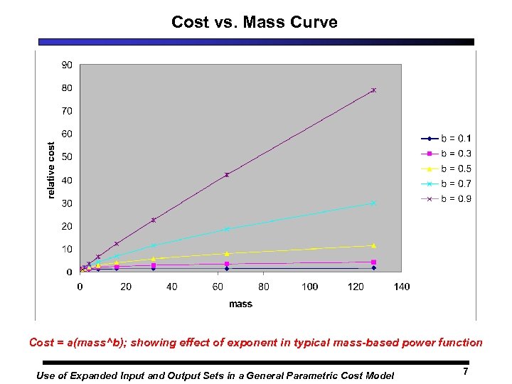Cost vs. Mass Curve Cost = a(mass^b); showing effect of exponent in typical mass-based power function Use of Expanded Input and Output Sets in a General Parametric Cost Model 7

More on mass-based general models • Strong non-linearity of equations with respect to size parameter limits capability to model at lower WBS input levels (see plot) • Mass has been eliminated in some general models – Example: PRICEM ™ Use of Expanded Input and Output Sets in a General Parametric Cost Model 8

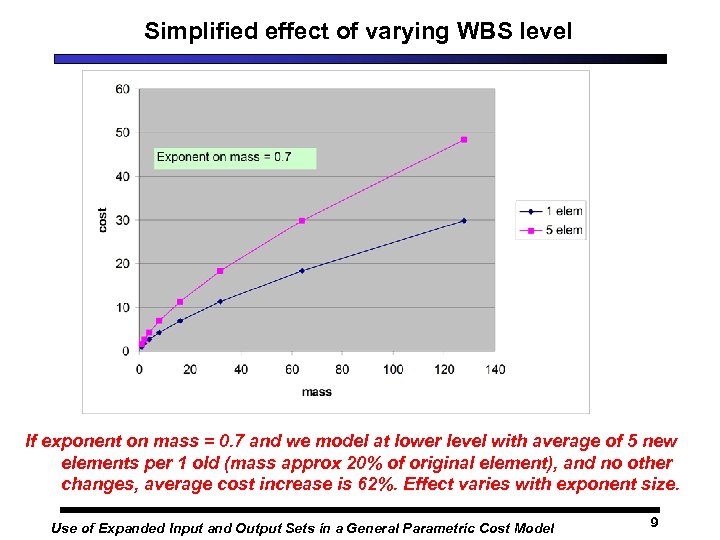Simplified effect of varying WBS level If exponent on mass = 0. 7 and we model at lower level with average of 5 new elements per 1 old (mass approx 20% of original element), and no other changes, average cost increase is 62%. Effect varies with exponent size. Use of Expanded Input and Output Sets in a General Parametric Cost Model 9

Inverse Example: Light-weighting • Degree of light-weighting (structure, optics) is often a design trade variable and typically has a large effect on cost and schedule that is inversely related to mass – With typical mass-based CER, results as mass varies are probably opposite to the observed cost trend – Use of non-mass parameters (hog-out, material, etc) may help, but effect of mass is (always? ) opposite to observed cost trend, therefore: • Effects of non-mass parameters must be exaggerated to compensate, or • Calibrations are needed, but are only good for a specified % of lightweighting • Worse still if % of light-weighting was not specified in calibration data • Material costs may also be off unless separate materials algorithm uses original, un-machined mass • Poor equation logic with respect to size limits the value and applicability of sensitivity analysis, ideally a key benefit of parametric modeling Use of Expanded Input and Output Sets in a General Parametric Cost Model 10

Brief history of development (1) • Identified a potential alternate size parameter – Experimented with number of parts (NP) from mechanical data • First np-based engineering equations – Started with engineer's rule of thumb for hours per drawing, adapted to full parameter set with NP as primary variable – New equation, using NP data from mechanical drawing sets, modeled labor hour trend in data well – Tested as alternate algorithm in existing models • Long period of use, development, refinement – – Learned to estimate, developed guidelines for NP Expanded use of NP in models Adapted approach to electronics (number of pins) Eventually used NP relationship as core engineering equation, developed general model around it Use of Expanded Input and Output Sets in a General Parametric Cost Model 11

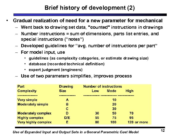Brief history of development (2) • Gradual realization of need for a new parameter for mechanical – Went back to drawing set data, "counted" instructions in drawings – Number instructions = sum of dimensions, parts list entries, and special instructions (“notes”) – Developed guidelines for “avg. number of instructions per part” – For model input, use • guidelines (as complexity categories, or estimate drawing size) • database (recorded technical definition) • expert judgment (engineers) – Use of two parameters simplifies, improves process Use of Expanded Input and Output Sets in a General Parametric Cost Model 12

Brief history of development (3) • Decompose output into phases; integrate with schedule calculations – Realized that much informal data exists to support allocation of cost to phases, as for software models – Started with conceptual prototype, gradually refined; still refining – Used standard development phases and simple assumptions to calculate resources per unit time • Simple level-of-effort assumptions, applied at low level, were determined to be more appropriate than distribution spreading functions used traditionally for high level calculations – Composite sum results vary with input assumptions; sometimes differ significantly from results obtained with traditional higher level functions, but in a reasonable way, according to schedule assumptions – Modeling of effect of schedule constraints on cost profile now possible Use of Expanded Input and Output Sets in a General Parametric Cost Model 13

Brief history of development (4) • More detail in output leads to more input changes – Allocation of prototypes, other associated parameters to phases – Probably more to go in this area • Beginning of common element database – So far a collection of elements from prior work, organized in subsystems as originally used. – More sophisticated approach not yet defined; structure needs to be considered carefully because much relevant information is in subsystem context (above element level). Use of Expanded Input and Output Sets in a General Parametric Cost Model 14

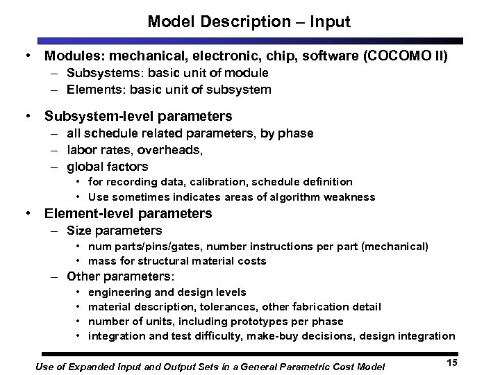Model Description – Input • Modules: mechanical, electronic, chip, software (COCOMO II) – Subsystems: basic unit of module – Elements: basic unit of subsystem • Subsystem-level parameters – all schedule related parameters, by phase – labor rates, overheads, – global factors • for recording data, calibration, schedule definition • Use sometimes indicates areas of algorithm weakness • Element-level parameters – Size parameters • num parts/pins/gates, number instructions per part (mechanical) • mass for structural material costs – Other parameters: • • engineering and design levels material description, tolerances, other fabrication detail number of units, including prototypes per phase integration and test difficulty, make-buy decisions, design integration Use of Expanded Input and Output Sets in a General Parametric Cost Model 15

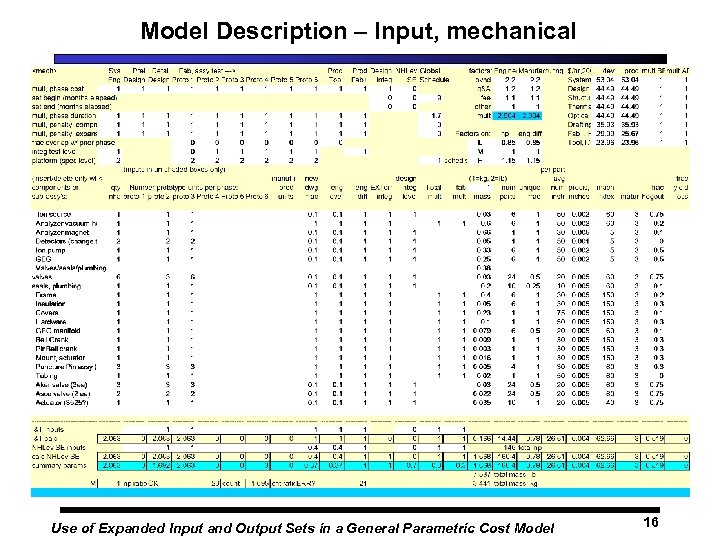Model Description – Input, mechanical Use of Expanded Input and Output Sets in a General Parametric Cost Model 16

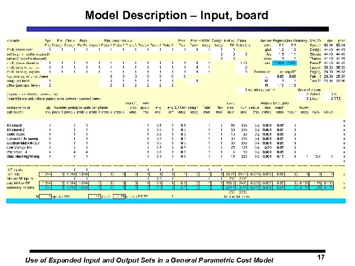Model Description – Input, board Use of Expanded Input and Output Sets in a General Parametric Cost Model 17

Model Description - Output • Basic model output is at the subsystem level and consists of – Hours, dollars and staffing levels – By functional elements – In discrete phases and uniform time units (months) • More granularity in input yields more detail in output • Detailed comparison by function, phase and time is possible at lowest subsystem level • Output is accumulated at higher levels – Hours or staffing levels, dollars – Summary and by month Use of Expanded Input and Output Sets in a General Parametric Cost Model 18

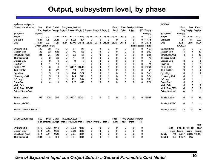Output, subsystem level, by phase Use of Expanded Input and Output Sets in a General Parametric Cost Model 19

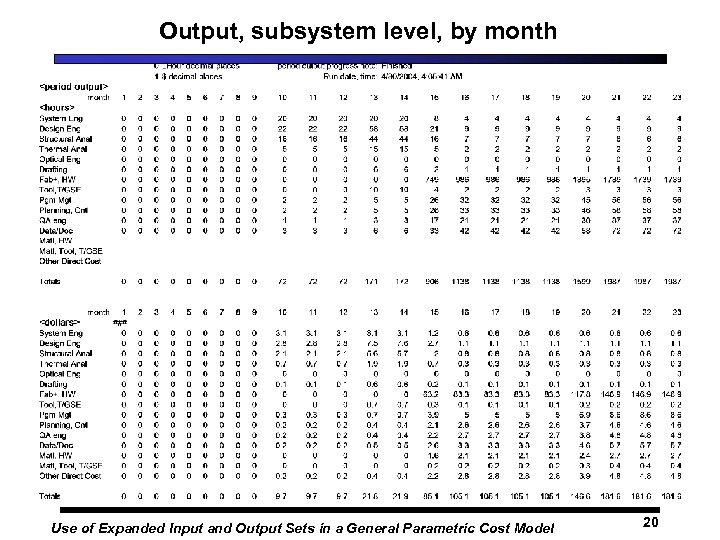Output, subsystem level, by month Use of Expanded Input and Output Sets in a General Parametric Cost Model 20

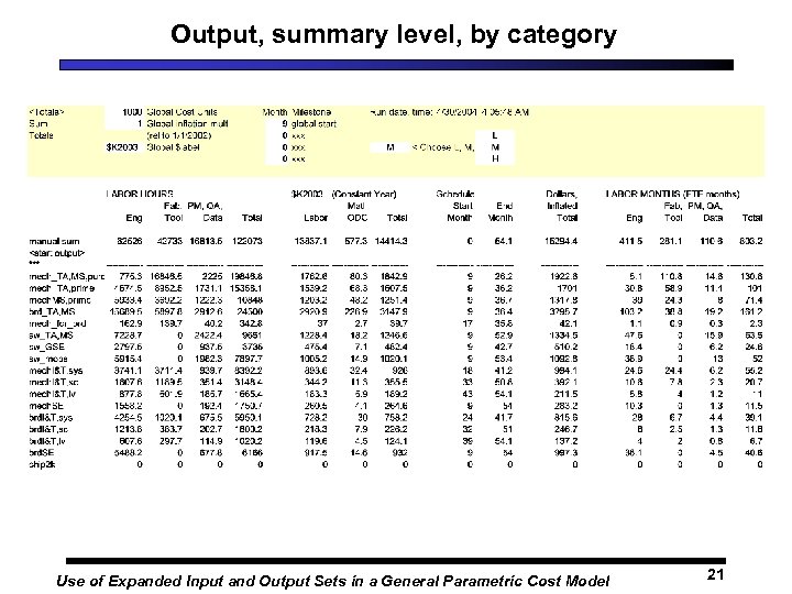Output, summary level, by category Use of Expanded Input and Output Sets in a General Parametric Cost Model 21

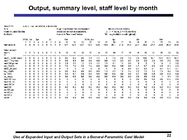Output, summary level, staff level by month Use of Expanded Input and Output Sets in a General Parametric Cost Model 22

Model Description – Algorithms (1) • Sources – Data from a variety of sources • Collected at as detailed a level as possible • Resources, schedule, definition (including drawing sets) • Interviews with project personnel – Expert judgment • Interviews with engineers in area of expertise – Other models, cost analysis literature • Secondary and generic algorithms, • logic (schedule, integration), etc. • Model maturity – Mechanical module is most developed and unique – Board module less well developed but has long heritage of use – Chip module less mature, not a primary tool, used to integrate estimates from other sources – Use of COCOMO II for software, with some adaptations for compatibility with other modules Use of Expanded Input and Output Sets in a General Parametric Cost Model 23

Model Description – Algorithms (2) • Core Engineering Equations (Mechanical) – Linear function of size parameters (num parts, num instructions per part) – Num drawings = num parts * num instructions/part * unique fraction * assembly drawing factor • (1 detail drawing per unique part, plus assembly drawings) • check on process is engineer’s estimate of drawings – Eng base = num drawings * fab cplx fac * platform fac * eng level * calibration fac • fabrication complexity factor is much less influential than in massbased models because size parameters are dominant • Board, chip modes are similar – board mode uses number of pins for size parameter – chip mode uses number of gates or transistors Use of Expanded Input and Output Sets in a General Parametric Cost Model 24

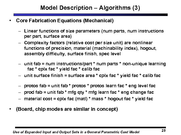Model Description – Algorithms (3) • Core Fabrication Equations (Mechanical) – Linear functions of size parameters (num parts, num instructions per part, surface area) – Complexity factors (relative cost per size unit) are nonlinear functions of precision, material (machinability index), hogout, assembly difficulty, surface finish, spec level – unit fab = num instructions/part * num parts * non-unique learning fac * cplx fac * yield fac * calib fac – unit surface finish = surface area * cplx fac * yield fac * calib fac – protos fab = unit fab * protos learn fac * eng level fac – prod fab = unit fab * mfg qty * mfg learn fac * eng change fac – material cost = cplx fac (matl) * mass * hogout fac * yield fac • (Board, chip modes are similar in concept) Use of Expanded Input and Output Sets in a General Parametric Cost Model 25

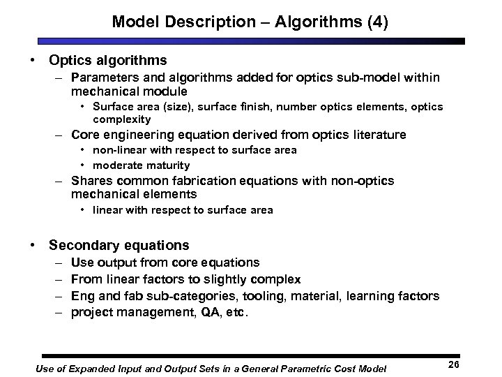Model Description – Algorithms (4) • Optics algorithms – Parameters and algorithms added for optics sub-model within mechanical module • Surface area (size), surface finish, number optics elements, optics complexity – Core engineering equation derived from optics literature • non-linear with respect to surface area • moderate maturity – Shares common fabrication equations with non-optics mechanical elements • linear with respect to surface area • Secondary equations – – Use output from core equations From linear factors to slightly complex Eng and fab sub-categories, tooling, material, learning factors project management, QA, etc. Use of Expanded Input and Output Sets in a General Parametric Cost Model 26

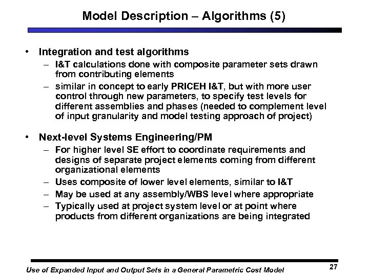Model Description – Algorithms (5) • Integration and test algorithms – I&T calculations done with composite parameter sets drawn from contributing elements – similar in concept to early PRICEH I&T, but with more user control through new parameters, to specify test levels for different assemblies and phases (needed to complement level of input granularity and model testing approach of project) • Next-level Systems Engineering/PM – For higher level SE effort to coordinate requirements and designs of separate project elements coming from different organizational elements – Uses composite of lower level elements, similar to I&T – May be used at any assembly/WBS level where appropriate – Typically used at project system level or at point where products from different organizations are being integrated Use of Expanded Input and Output Sets in a General Parametric Cost Model 27

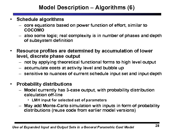Model Description – Algorithms (6) • Schedule algorithms – core equations based on power function of effort, similar to COCOMO – also some logic; real complexity is in number of phases and depth of subsystem definition • Resource profiles are determined by accumulation of lower level, discrete phase output – not by applying theoretical functional forms to high level output – accumulate costs at activity level and bubble up – sensitive to nuances of current schedule input set and input depth • Probability distributions – Model currently has 3 -case output, with probability distribution calculation off-line • LMH input for selected set of parameters – May add Monte-Carlo simulation with inputs in form of probability distributions (reuse code from earlier model versions) Use of Expanded Input and Output Sets in a General Parametric Cost Model 28

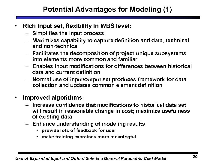Potential Advantages for Modeling (1) • Rich input set, flexibility in WBS level: – Simplifies the input process – Maximizes capability to capture definition and data, technical and non-technical – Facilitates the decomposition of project-unique subsystems into elements more common and familiar – Enables input modifications for differences between historical data and current definition – Normal use of input/output set produces framework for data collection and updates common element definition • Improved algorithms – Increase confidence that modifications to historical data set will result in reasonable change in cost; maximize usefulness of existing data – Enhance understanding of modeling results • provide lots of feedback for user • make training exercises more meaningful Use of Expanded Input and Output Sets in a General Parametric Cost Model 29

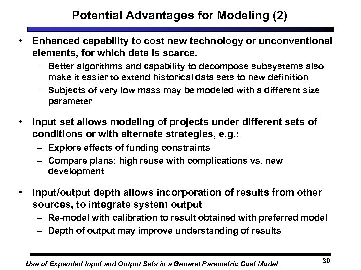Potential Advantages for Modeling (2) • Enhanced capability to cost new technology or unconventional elements, for which data is scarce. – Better algorithms and capability to decompose subsystems also make it easier to extend historical data sets to new definition – Subjects of very low mass may be modeled with a different size parameter • Input set allows modeling of projects under different sets of conditions or with alternate strategies, e. g. : – Explore effects of funding constraints – Compare plans: high reuse with complications vs. new development • Input/output depth allows incorporation of results from other sources, to integrate system output – Re-model with calibration to result obtained with preferred model – Depth of output may improve understanding of results Use of Expanded Input and Output Sets in a General Parametric Cost Model 30

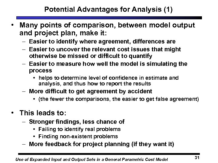Potential Advantages for Analysis (1) • Many points of comparison, between model output and project plan, make it: – Easier to identify where agreement, differences are – Easier to uncover the relevant cost issues that might otherwise be missed or difficult to quantify – Easier to measure how well the model is simulating the process • helps to determine level of confidence in estimate and analysis, and thus how to report the results – More difficult to get agreement by accident • (the fewer the comparisons, the easier to get false agreement) • This leads to: – Stronger findings, less chance of • Failing to identify real problems • Finding non-existent problems – More feedback for project planning (if they want it) Use of Expanded Input and Output Sets in a General Parametric Cost Model 31

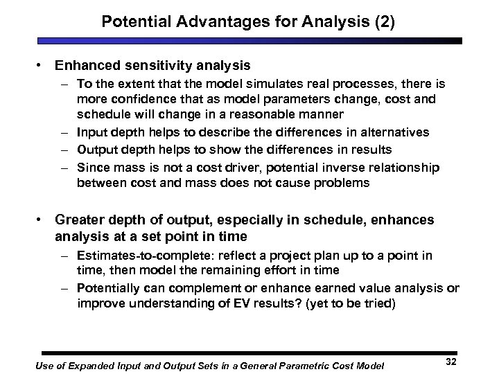Potential Advantages for Analysis (2) • Enhanced sensitivity analysis – To the extent that the model simulates real processes, there is more confidence that as model parameters change, cost and schedule will change in a reasonable manner – Input depth helps to describe the differences in alternatives – Output depth helps to show the differences in results – Since mass is not a cost driver, potential inverse relationship between cost and mass does not cause problems • Greater depth of output, especially in schedule, enhances analysis at a set point in time – Estimates-to-complete: reflect a project plan up to a point in time, then model the remaining effort in time – Potentially can complement or enhance earned value analysis or improve understanding of EV results? (yet to be tried) Use of Expanded Input and Output Sets in a General Parametric Cost Model 32

Example 1: Time-phased output • Spacecraft development cost estimate • Chart 1: cum probability curve • Chart 2: time-phased probability Use of Expanded Input and Output Sets in a General Parametric Cost Model 33

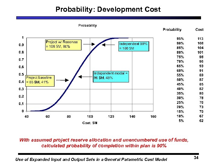Probability: Development Cost With assumed project reserve allocation and unencumbered use of funds, calculated probability of completion within plan is 90% Use of Expanded Input and Output Sets in a General Parametric Cost Model 34

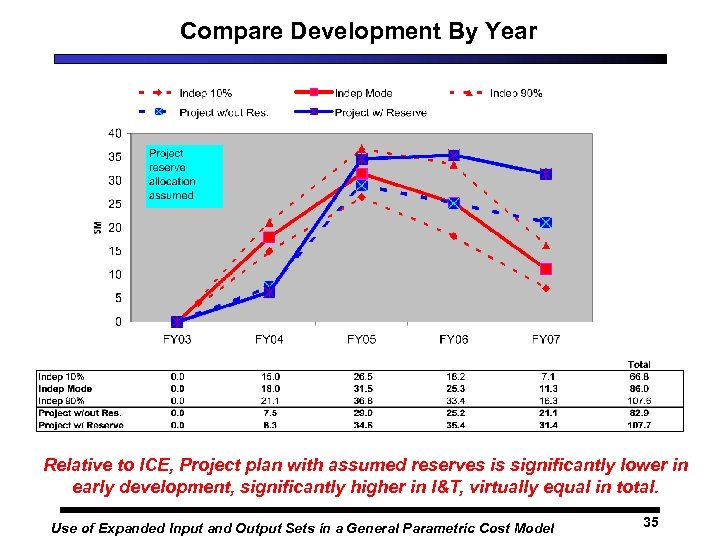Compare Development By Year Relative to ICE, Project plan with assumed reserves is significantly lower in early development, significantly higher in I&T, virtually equal in total. Use of Expanded Input and Output Sets in a General Parametric Cost Model 35

Example 1: Time-phased output analysis • Chart 1: cum probability curve – Shows no significant difference between project plan and parametric estimate • Chart 2: time-phased probability – Shows significant difference: resources available to project in early phases are significantly less than levels suggested by cost modeling • Difference was mostly explained by externally imposed constraints on early funding for project. • Review team finding: – “Probability of problems resulting from inadequate early definition may be higher than desired. ” – (Project mission success potentially at increased risk due to inadequate early funding) Use of Expanded Input and Output Sets in a General Parametric Cost Model 36

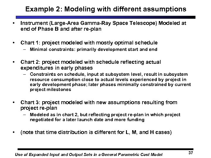Example 2: Modeling with different assumptions • Instrument (Large-Area Gamma-Ray Space Telescope) Modeled at end of Phase B and after re-plan • Chart 1: project modeled with mostly optimal schedule – Minimal constraints: primarily development start and end • Chart 2: project modeled with schedule reflecting actual expenditures in early phases – Constraints on schedule, input at subsystem level, result in subsystem resource consumption close to actual levels experienced by project in early development phase; later phases minimally constrained by current project milestones • Chart 3: project modeled with new assumptions resulting from project re-plan – Modeled as in chart 2, but reflecting project re-plan in which project negotiated for a later launch date and more funding • (note that time distribution is different for L, M, and H cases) Use of Expanded Input and Output Sets in a General Parametric Cost Model 37

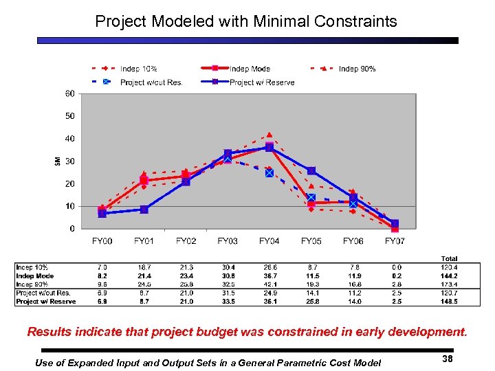Project Modeled with Minimal Constraints Results indicate that project budget was constrained in early development. Use of Expanded Input and Output Sets in a General Parametric Cost Model 38

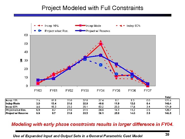Project Modeled with Full Constraints Modeling with early phase constraints results in larger difference in FY 04. Use of Expanded Input and Output Sets in a General Parametric Cost Model 39

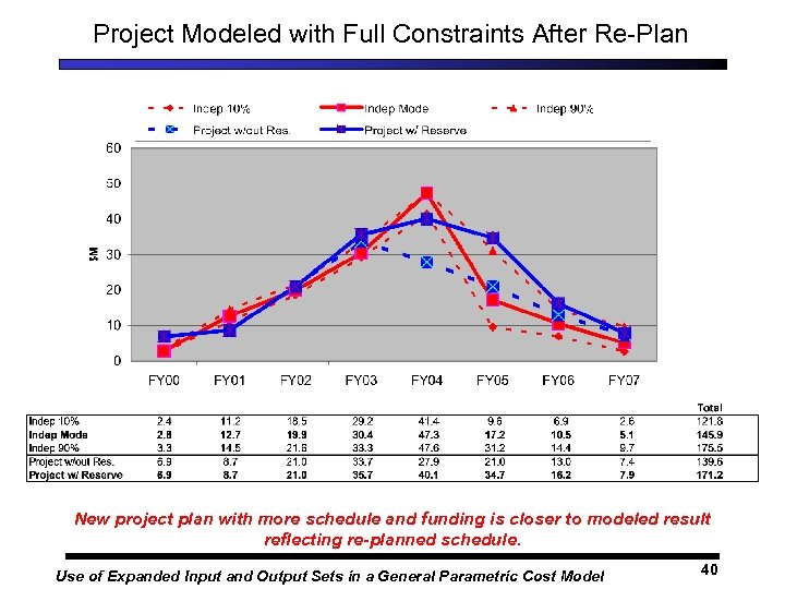Project Modeled with Full Constraints After Re-Plan New project plan with more schedule and funding is closer to modeled result reflecting re-planned schedule. Use of Expanded Input and Output Sets in a General Parametric Cost Model 40

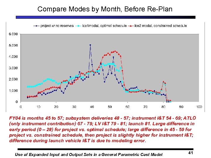Compare Modes by Month, Before Re-Plan FY 04 is months 45 to 57; subsystem deliveries 48 - 57; instrument I&T 54 - 69; ATLO (only instrument contribution) 67 - 79; LV I&T 79 - 81; launch 81. Large difference in early period (0 – 28) for project vs. optimal schedule; large difference in 45 - 59 for project vs. constrained schedule, then project is slightly higher for instrument I&T; difference during launch vehicle I&T is due to modeling error. Use of Expanded Input and Output Sets in a General Parametric Cost Model 41

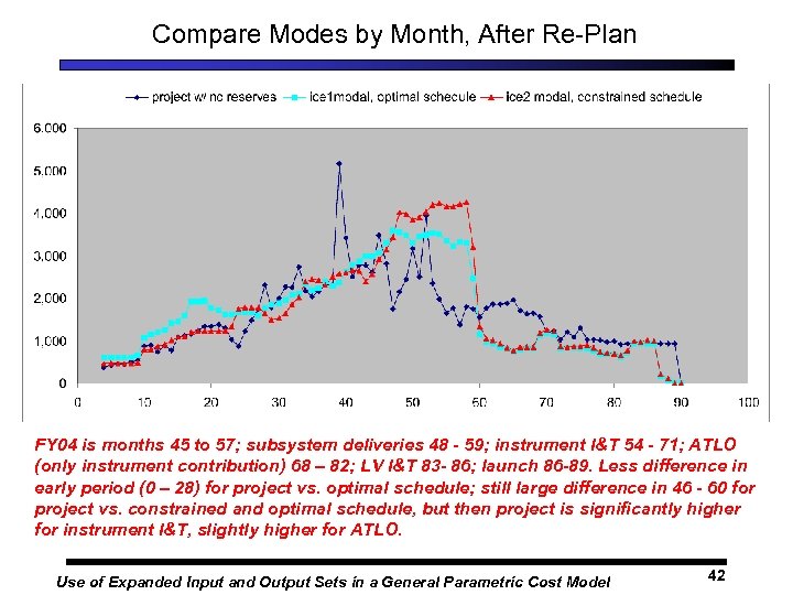Compare Modes by Month, After Re-Plan FY 04 is months 45 to 57; subsystem deliveries 48 - 59; instrument I&T 54 - 71; ATLO (only instrument contribution) 68 – 82; LV I&T 83 - 86; launch 86 -89. Less difference in early period (0 – 28) for project vs. optimal schedule; still large difference in 46 - 60 for project vs. constrained and optimal schedule, but then project is significantly higher for instrument I&T, slightly higher for ATLO. Use of Expanded Input and Output Sets in a General Parametric Cost Model 42

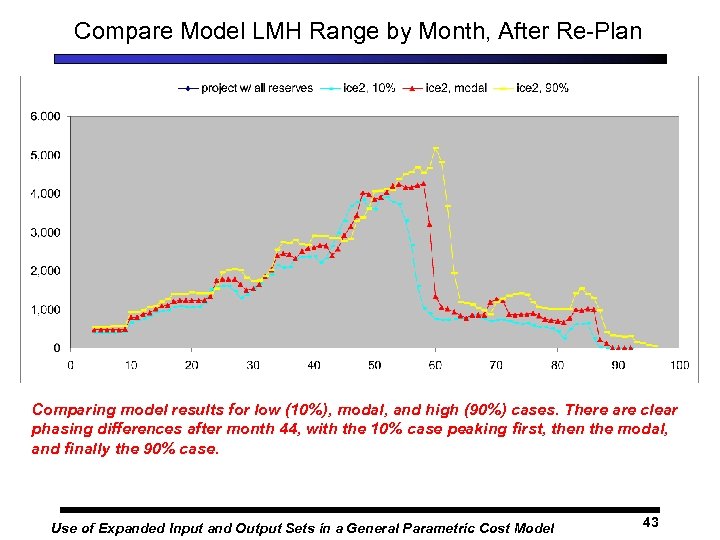Compare Model LMH Range by Month, After Re-Plan Comparing model results for low (10%), modal, and high (90%) cases. There are clear phasing differences after month 44, with the 10% case peaking first, then the modal, and finally the 90% case. Use of Expanded Input and Output Sets in a General Parametric Cost Model 43

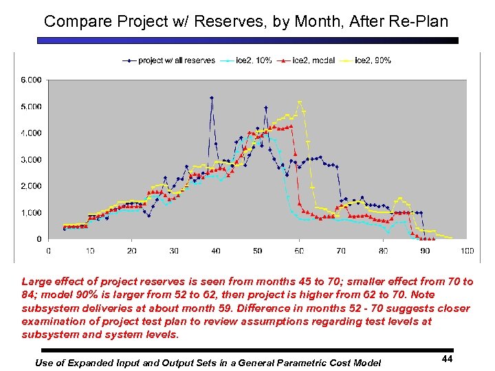Compare Project w/ Reserves, by Month, After Re-Plan Large effect of project reserves is seen from months 45 to 70; smaller effect from 70 to 84; model 90% is larger from 52 to 62, then project is higher from 62 to 70. Note subsystem deliveries at about month 59. Difference in months 52 - 70 suggests closer examination of project test plan to review assumptions regarding test levels at subsystem and system levels. Use of Expanded Input and Output Sets in a General Parametric Cost Model 44

Advantages for Model Development • Rich input set increases the usefulness of available definition – Capability to define at lower WBS levels allows small subsets of projects, for which good data is available, to be modeled, thereby increasing usefulness of data – Deep input set allows more historical technical definition to be captured in the model • Rich output set increases the usefulness of available cost/resources data – Many points of comparison allow better matching with cost data • increase the capability to crosscheck, validate, or calibrate results against known quantities – Detailed output generates more feedback, exposes modeling errors, speeds up model development • Use of improved size parameters has resulted in more linear functional forms, which have numerous advantages for modeling and for development Use of Expanded Input and Output Sets in a General Parametric Cost Model 45

Practical implications for use of model • To use the model well, user must become familiar with new size parameters – Process is somewhat like instruction count estimating in use of software models • As with software instructions, process increases analyst’s knowledge of cause and effect in cost analysis – Engineers are familiar with these parameters, but analyst must also become familiar with them, more or less according to level of interaction with engineers • Building data base lessens dependence on engineers, increases knowledge – Initially requires more time to learn a new technique • After learning the process, there is a time trade-off: spend more time on new size input, but less time on calibration or "complexity" values Use of Expanded Input and Output Sets in a General Parametric Cost Model 46

Author Bias: Value of information • An analysis is only as good as the information that went into it. – You don't get something for nothing. If you want more confidence in cost and schedule estimates, you have to consider more information in the analysis. – To the extent that you are able to effectively include relevant information in your analysis, the value of the result increases and the uncertainty decreases. Use of Expanded Input and Output Sets in a General Parametric Cost Model 47

Author Bias: Use of Informal Logic • Define informal logic (IL): relationship that has good basis in informal observation but has not been empirically verified – Tools that model complex processes necessarily supplement empirical knowledge with IL, in order to model the complexity of the system – Complex models are built around prevailing hypotheses • Weather, economics, etc. • Resource consumption (cost) is a complex process • Also, cost data (even the best) is not experimental data, but really is observation (field) data • Therefore cost models need to be supplemented with IL, and there is a wealth of informal data available for this purpose. • Unofficial data, expert opinion, context logic • Unless you are clueless, plugging a gap with your best guess is better than ignoring the issue; ignoring it amounts to making implicit or unknown assumptions about it; including it insures that you know why you got what you got • Progress is made by creating and testing hypotheses Use of Expanded Input and Output Sets in a General Parametric Cost Model 48

End Use of Expanded Input and Output Sets in a General Parametric Cost Model 49