UNIVERSITY CERTIFICATE IN ECONOMETRICS 2017 Edition

UNIVERSITY CERTIFICATE IN ECONOMETRICS 2017 · Edition 2 Course : Microeconometrics for policy evaluation Part 2 - Policy evaluation/treatment analysis Vincent Vandenberghe

OUTLINE 1. 2. 3. 4. Introduction The endogeneity problem Experimental methods Quasi-experimental methods • • Short panel analysis (day 1) Policy evaluation/treatment analysis (day 2) § Difference-in-Difference estimation: § Treatment effects with non-experimental data using (repeated) cross-sectional data § The canonical Di. D estimator § Assessing the common trend assumption § Relaxing the common trend assumption: from Di. D § Propensity score matching § Matching over a single (propensity) score § Matching algorithms (nearest neighborhood, caliper, Kernel) § Combining Di. D and propensity score matching

OUTLINE Main Stata commands 1. reg 2. psmatch 2 3. teffects 4. diff

USEFUL REFERENCES Cameron, A. C. & Trivedi, P. K. (2010). Microeconometrics using Stata. College Station: Stata Press.

Policy_eval. Folder MATERIAL @ YOUR DISPOSAL MOODLE@UCL: LECME 2 FC TOPIC 2 Policy_eval ECcourse 2. ppt Code…Stata_code #2 EC_PSMATCH. do #2 EC_Extra. do #2 EC_Ex_corr. do #2 EC_Ex. do #2 EC_Di. D. do #2 EC_data. do __________ (+ corrected version at the end) Data. zip the various data sets @ your disposal via the web: https: //perso. uclouvain. be/vincent. vandenberghe/Stata_EC 1. html 5

4. QUASI-EXPERIMENTAL METHODS: POLICY EVALUATION 4. 1. Difference-in-Differences (or two-way fixed effects) Let’s think about a simple evaluation of a policy (treatment) If we have data on a bunch of people right before the policy is enacted and on the same group of people after it is enacted. How can we try to identify the effect Suppose we have two years (the shortest possible panel) of data t=0 and t=1 and that the policy/treatment is enacted in between We could try to identify the effect by simply looking at y before and after the policy. That is we can identify the effect by resorting to first differences 6

[Eq 6] yt = β TRt + Z + ut where TRt= 1 if t=1 and 0 if t=0, Z is the unobserved fixed effect caracterizing the treated, potentially correlated with treatment One way of dealing with Z is to resort to first differences [Eq 7] E(y 1)-E(y 0)= β The problem with this “difference model” is that it attributes any changes in time to the policy Suppose something else happened between t=0 and t=1 other than just the program (eg. an economic recession/boom) We will attribute whatever that is to the program/treatment 7

How to solve the problem? Simply adding a time dummy (t) would not help us separate the time effect from the treatment effect (ie. perfect collinearity=> TRt=t) Rather suppose we have two groups: - People who are affected by the policy changes (D=1) - People who are not affected by the policy change (D=0) => the controls 8

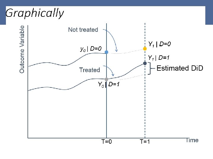
We can think of using the control to pick up the time changes: [Eq. 8] E(y 1|D=0) - E(y 0|D=0) Then we can estimate our policy effect as a “difference in (time-driven) differences” (Di. D) between the treated and the control group [Eq. 9] [E(y 1|D=1) - E(y 0|D=1) ]− [E(y 1|D=0) - E(y 0|D=0) ] 9

Algebraically [Eq. 10] yt= α + D*t + lt + δD + ut Remember : D=0 if not treated and D=1 if treated (with ZD=1 =α + δ; ZD=0 =α) [E(y 1|D=1) - E(y 0|D=1) ]− [E(y 1|D=0) - E(y 0|D=0) ] =[α + + l+ δ – α – δ ]− [α +l -α ] = So estimating by OLS in the above equation will deliver the treatment effect as Di. D 11

Key assumption : the control group (D=0) identifies the time path (ie. growth) of outcomes – the trend - that would have happened to the treated (D=1) in the absence of the treatment ó control & treated outcome are assumed to be characterized by the same trend (common trend assumption) ex ante ó Identification of the impact of treatment relies on the change of trend specific to the treated group ó In practice, the common-trend assumption prior to treatment requires a certain element of geographical and political proximity ó It can be tested if panels contains several periods of observation prior to treatment 12

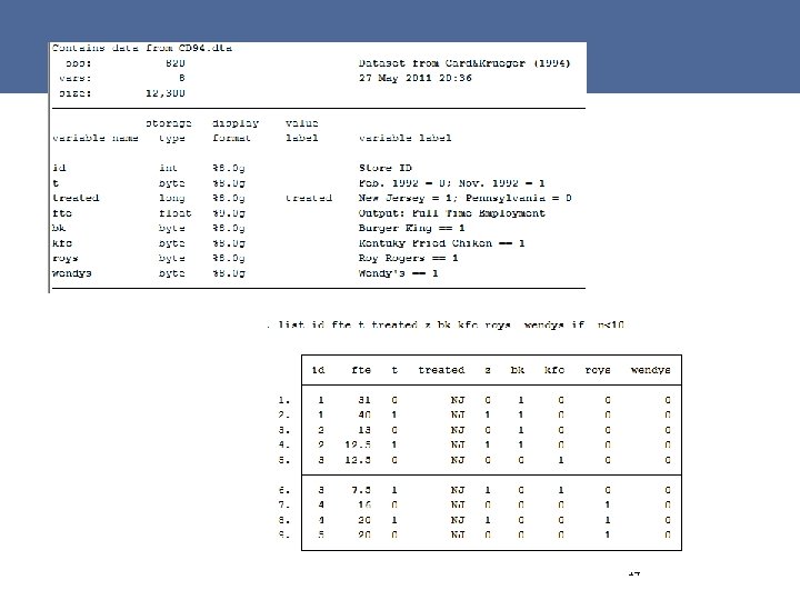
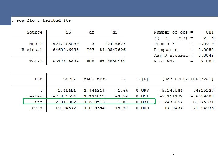
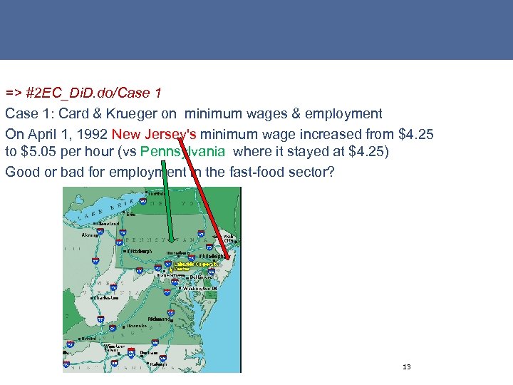=> #2 EC_Di. D. do/Case 1: Card & Krueger on minimum wages & employment On April 1, 1992 New Jersey's minimum wage increased from $4. 25 to $5. 05 per hour (vs Pennsylvania where it stayed at $4. 25) Good or bad for employment in the fast-food sector? 13

14

15

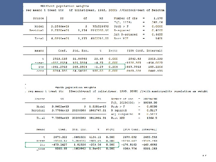
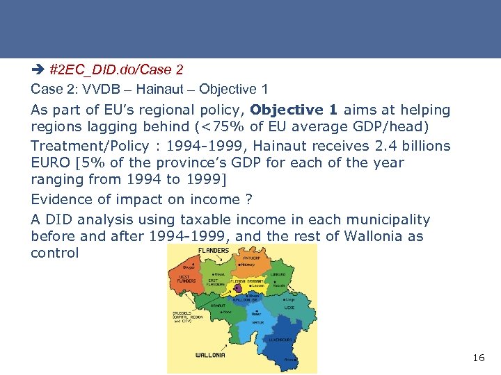è #2 EC_DID. do/Case 2: VVDB – Hainaut – Objective 1 As part of EU’s regional policy, Objective 1 aims at helping regions lagging behind (<75% of EU average GDP/head) Treatment/Policy : 1994 -1999, Hainaut receives 2. 4 billions EURO [5% of the province’s GDP for each of the year ranging from 1994 to 1999] Evidence of impact on income ? A DID analysis using taxable income in each municipality before and after 1994 -1999, and the rest of Wallonia as control 16

17

If you have several time periods before treatment begins…. - You can test the crucial common trend/parallelism assumption; simply by estimating Di. D using two pretreatment periods 18

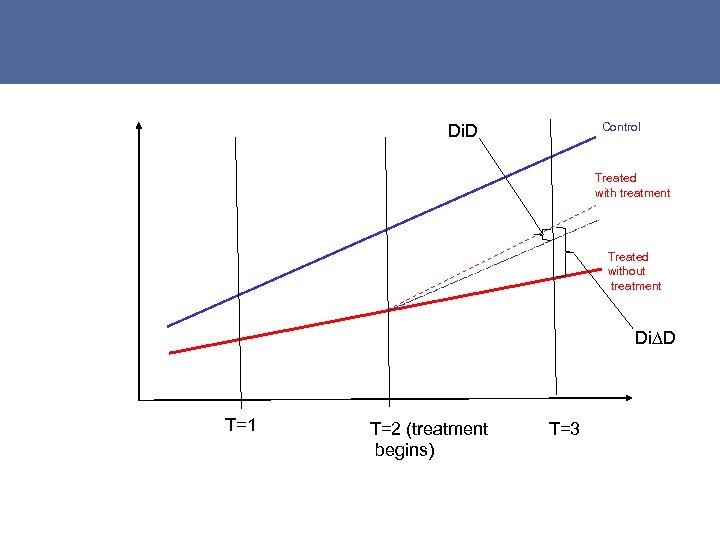
- You can relax the parallel path assumption, assume parallel growth and estimate “treatment” as differences-in-(differencein-difference) (i. e. change in growth rate differences instead of level differences over time) 19

Control Di. D Treated with treatment Treated without treatment Di∆D T=1 T=2 (treatment begins) T=3

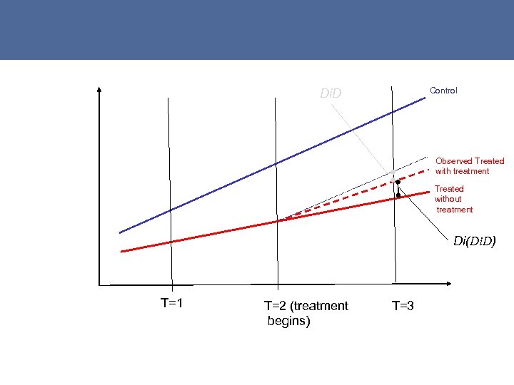Control Di. D Observed Treated with treatment Treated without treatment Di(Di. D) T=1 T=2 (treatment begins) T=3

[Eq. 11] Yt= γ + γ 2 T 2 + γ 3 T 3 + γD D + γD 2 D. T 2 + γD 3 D. T 3 Estimators = Di. D 2/1= γD 2+γD-γD=γD 2 reflecting the « normal » growth rate difference Di. D 3/2=(γD 3+γD)-(γD 2 +γD)=γD 3 - γD 2 ; Di(Di. D)= Di. D 3/2 - Di. D 2/1= (γD 3 -γD 2)- γD 2= γD 3 - 2γD 2 D=0; Control Di. D 3/2 γ 3 γ 2 γ γD 3 2γD 2 γD γD γD Observed D=1; Treated with treatment D=1, Treated without treatment 2 γD T=1 Di(Di. D) T=2 (treatment begins) T=3 #2 EC_ex. do/Ex 1

4. 2. Propensity score matching methods In non-experimental economic data, we observe whether “individuals” were treated or not, but in the absence of random assignment, we must be concerned with differences between the treated and non-treated One very appealing idea is to match “individuals” with maximal similarity 23

With a single measure (e. g. X=education), we can readily compute a measure of distance between a treated unit and each candidate match. With multiple measures defining similarity, how are we to balance similarity along each of those dimensions (e. g. : X=education, wealth, #siblings…. )? Propensity score matching (PSM): match treated and untreated observations on the estimated probability of being treated (propensity score). P(X) = Pr (D=1|X) with D=1, 0 indicates (non)treatment => Key idea : rather than matching on all values of the variables, individual units can be matched solely on the basis of their propensity to be treated P(X) 24

Advantages of PSM - Solves the “dimensionaliy” problem • balances treatment and control groups on a large number of covariates(X) without losing a large number of observations • If treatment & control were balanced one at a time, large numbers of observations would be needed = > #X +1 increases the minimum necessary # of obs. geometrically 25

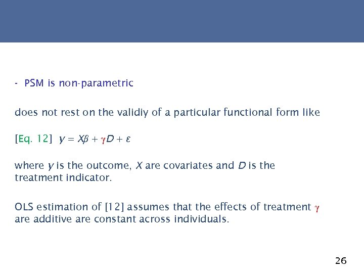- PSM is non-parametric does not rest on the validiy of a particular functional form like [Eq. 12] y = Xβ + γD + ε where y is the outcome, X are covariates and D is the treatment indicator. OLS estimation of [12] assumes that the effects of treatment γ are additive are constant across individuals. 26

PSM limitations - Conditional independence: PSM validity rests on [Eq. 13] (Y 1, Y 0) ⊥ D|X where Y 1, Y 0 denote treated/control potential outcomes under treatment [and ⊥ statistical independence]. Controlling for X is ‘as good as random. ’ This assumption is also known as selection on observables - Common support: there is sufficient overlap in propensity scores of treated and untreated units to find good matches 27

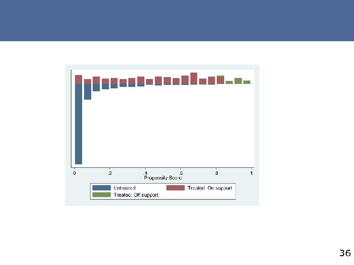
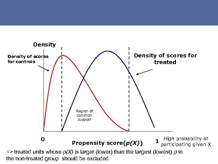Density of scores for treated Density of scores for controls Region of common support 0 Propensity score(p(X)) 1 High probability of participating given X => treated units whose p(X) is larger (lower) than the largest (lowest) p in the non-treated group should be excluded

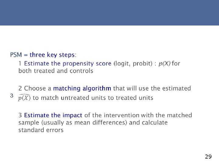3 29

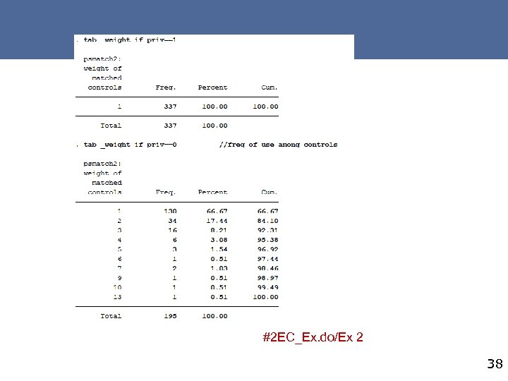
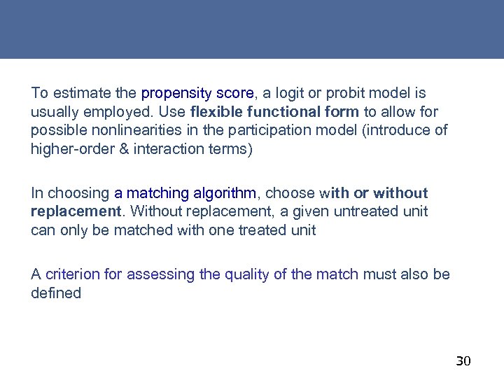To estimate the propensity score, a logit or probit model is usually employed. Use flexible functional form to allow for possible nonlinearities in the participation model (introduce of higher-order & interaction terms) In choosing a matching algorithm, choose with or without replacement. Without replacement, a given untreated unit can only be matched with one treated unit A criterion for assessing the quality of the match must also be defined 30

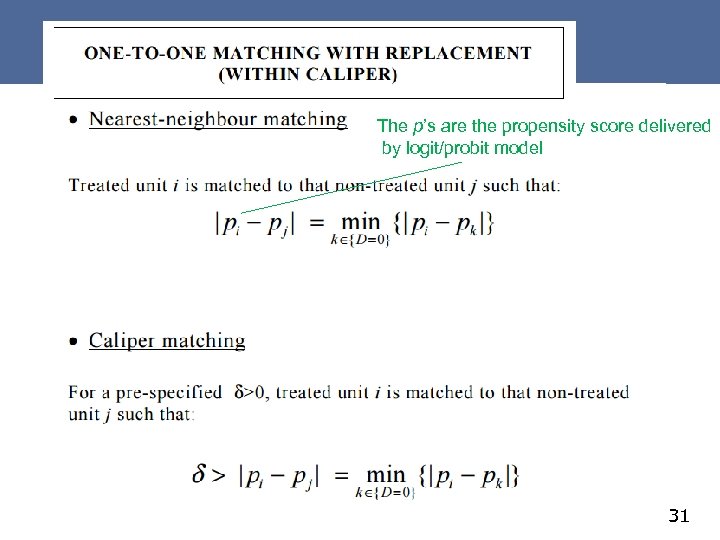The p’s are the propensity score delivered by logit/probit model 31

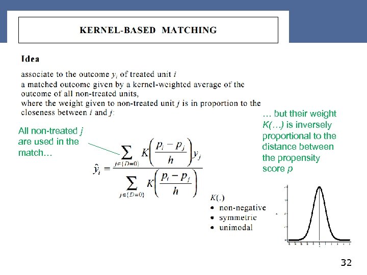All non-treated j are used in the match… … but their weight K(…) is inversely proportional to the distance between the propensity score p 32

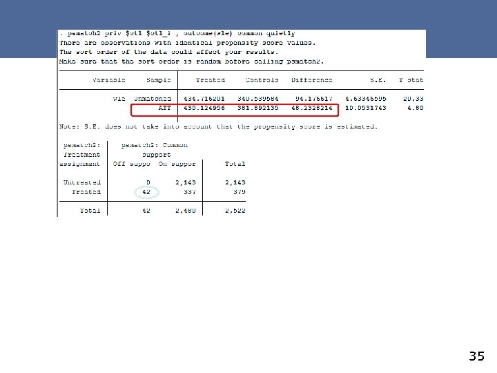
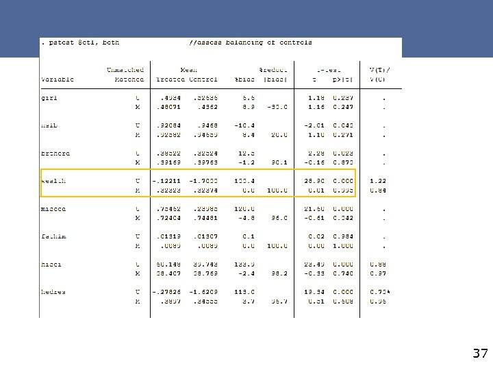
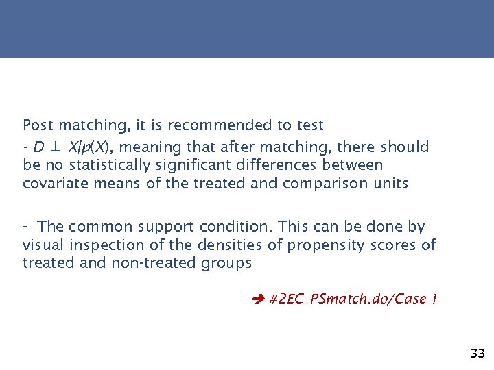Post matching, it is recommended to test - D ⊥ X|p(X), meaning that after matching, there should be no statistically significant differences between covariate means of the treated and comparison units - The common support condition. This can be done by visual inspection of the densities of propensity scores of treated and non-treated groups #2 EC_PSmatch. do/Case 1 33

34

35

36

37

#2 EC_Ex. do/Ex 2 38

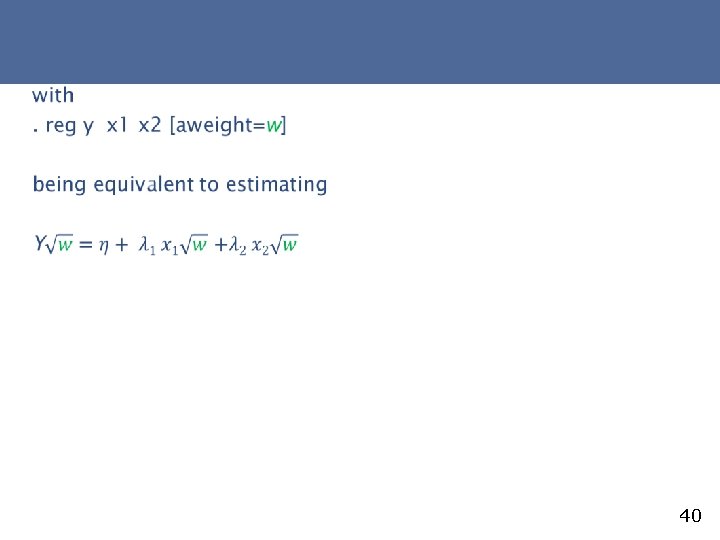
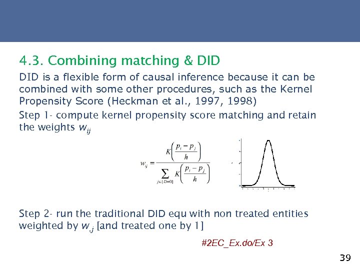4. 3. Combining matching & DID is a flexible form of causal inference because it can be combined with some other procedures, such as the Kernel Propensity Score (Heckman et al. , 1997, 1998) Step 1 - compute kernel propensity score matching and retain the weights wij Step 2 - run the traditional DID equ with non treated entities weighted by w. j [and treated one by 1] #2 EC_Ex. do/Ex 3 39

40