Unit 6 Starters Starter 11 1 1

Unit 6 Starters

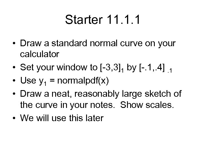Starter 11. 1. 1 • Draw a standard normal curve on your calculator • Set your window to [-3, 3]1 by [-. 1, . 4]. 1 • Use y 1 = normalpdf(x) • Draw a neat, reasonably large sketch of the curve in your notes. Show scales. • We will use this later

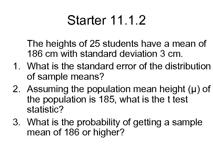Starter 11. 1. 2 The heights of 25 students have a mean of 186 cm with standard deviation 3 cm. 1. What is the standard error of the distribution of sample means? 2. Assuming the population mean height (µ) of the population is 185, what is the t test statistic? 3. What is the probability of getting a sample mean of 186 or higher?

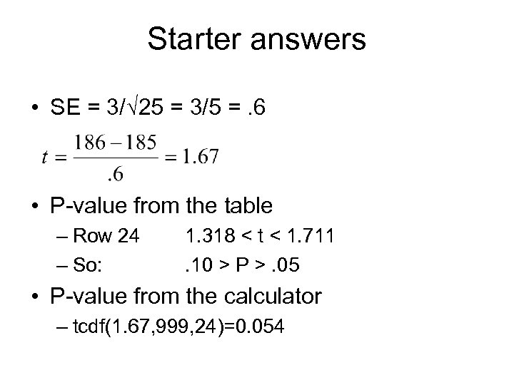Starter answers • SE = 3/√ 25 = 3/5 =. 6 • P-value from the table – Row 24 – So: 1. 318 < t < 1. 711. 10 > P >. 05 • P-value from the calculator – tcdf(1. 67, 999, 24)=0. 054

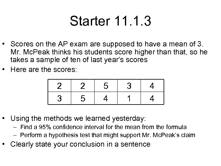Starter 11. 1. 3 • Scores on the AP exam are supposed to have a mean of 3. Mr. Mc. Peak thinks his students score higher than that, so he takes a sample of ten of last year’s scores • Here are the scores: 2 3 2 5 5 4 3 1 4 4 • Using the methods we learned yesterday: – Find a 95% confidence interval for the mean from the formula – Perform a hypothesis test that might support Mr. Mc. Peak’s claim • Clearly state your conclusion in a sentence

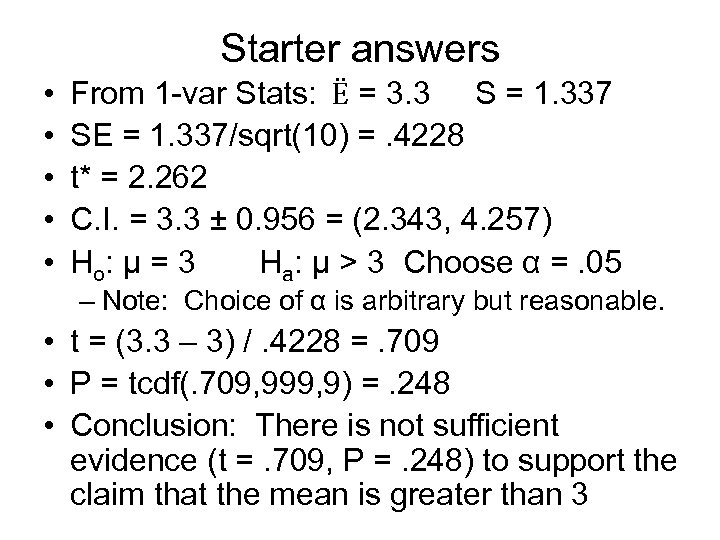Starter answers • • • From 1 -var Stats: Ë = 3. 3 S = 1. 337 SE = 1. 337/sqrt(10) =. 4228 t* = 2. 262 C. I. = 3. 3 ± 0. 956 = (2. 343, 4. 257) H o: μ = 3 Ha: μ > 3 Choose α =. 05 – Note: Choice of α is arbitrary but reasonable. • t = (3. 3 – 3) /. 4228 =. 709 • P = tcdf(. 709, 999, 9) =. 248 • Conclusion: There is not sufficient evidence (t =. 709, P =. 248) to support the claim that the mean is greater than 3

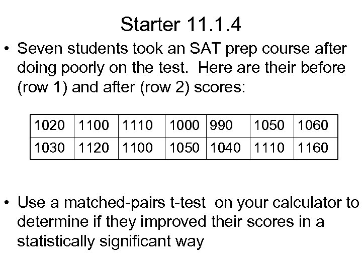Starter 11. 1. 4 • Seven students took an SAT prep course after doing poorly on the test. Here are their before (row 1) and after (row 2) scores: 1020 1100 1110 1000 990 1050 1060 1030 1120 1100 1050 1040 1110 1160 • Use a matched-pairs t-test on your calculator to determine if they improved their scores in a statistically significant way

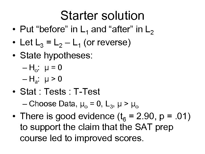Starter solution • Put “before” in L 1 and “after” in L 2 • Let L 3 = L 2 – L 1 (or reverse) • State hypotheses: – H o: μ = 0 – H a: μ > 0 • Stat : Tests : T-Test – Choose Data, μo = 0, L 3, μ > μo • There is good evidence (t 6 = 2. 90, p =. 01) to support the claim that the SAT prep course led to improved scores.

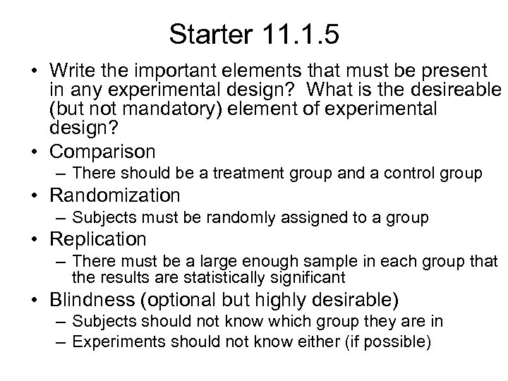Starter 11. 1. 5 • Write the important elements that must be present in any experimental design? What is the desireable (but not mandatory) element of experimental design? • Comparison – There should be a treatment group and a control group • Randomization – Subjects must be randomly assigned to a group • Replication – There must be a large enough sample in each group that the results are statistically significant • Blindness (optional but highly desirable) – Subjects should not know which group they are in – Experiments should not know either (if possible)

Starter 11. 2. 1 • Write the assumptions that underlie the use of the t test. • Which assumption is so important you can’t work without it? • What is the best way to tell if the distribution assumption is met?

Starter Solution • The two main assumptions we need are: – The sample came from a valid SRS of the population. – The population is approximately normally distributed. • We can’t do anything without a valid SRS. • Plot the data to see if they are approximately normal. – Note that if sample size is large we can live with skewness or outliers.

Starter 11. 2. 2 • In the early eighties, a large group of 13 year olds were given the SAT. Verbal results were nearly identical, but there was a real difference in the math results. Here are the facts: – 19, 883 boys had a mean score of 416 with standard deviation of 87 – 19, 937 girls had a mean score of 386 with a standard deviation of 74 • Use the formula to state a 99% confidence interval for the mean difference of scores between ALL boys and girls.

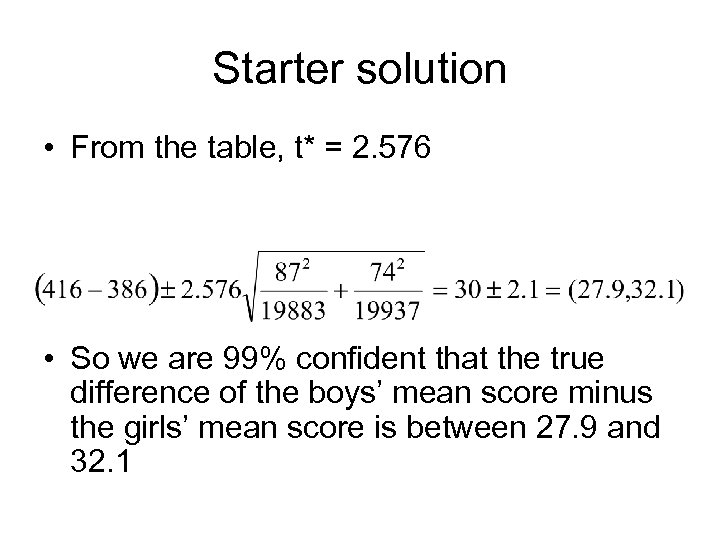Starter solution • From the table, t* = 2. 576 • So we are 99% confident that the true difference of the boys’ mean score minus the girls’ mean score is between 27. 9 and 32. 1

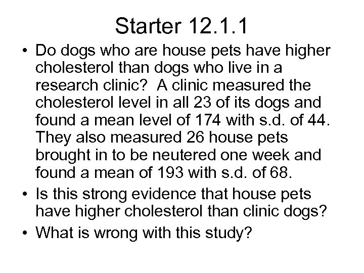Starter 12. 1. 1 • Do dogs who are house pets have higher cholesterol than dogs who live in a research clinic? A clinic measured the cholesterol level in all 23 of its dogs and found a mean level of 174 with s. d. of 44. They also measured 26 house pets brought in to be neutered one week and found a mean of 193 with s. d. of 68. • Is this strong evidence that house pets have higher cholesterol than clinic dogs? • What is wrong with this study?

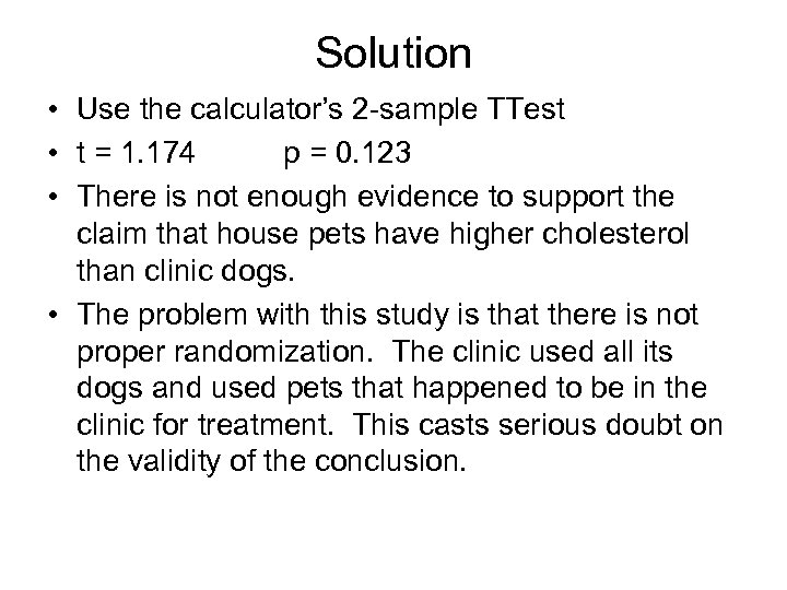Solution • Use the calculator’s 2 -sample TTest • t = 1. 174 p = 0. 123 • There is not enough evidence to support the claim that house pets have higher cholesterol than clinic dogs. • The problem with this study is that there is not proper randomization. The clinic used all its dogs and used pets that happened to be in the clinic for treatment. This casts serious doubt on the validity of the conclusion.

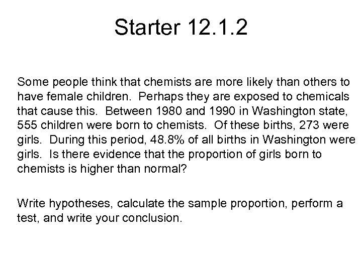Starter 12. 1. 2 Some people think that chemists are more likely than others to have female children. Perhaps they are exposed to chemicals that cause this. Between 1980 and 1990 in Washington state, 555 children were born to chemists. Of these births, 273 were girls. During this period, 48. 8% of all births in Washington were girls. Is there evidence that the proportion of girls born to chemists is higher than normal? Write hypotheses, calculate the sample proportion, perform a test, and write your conclusion.

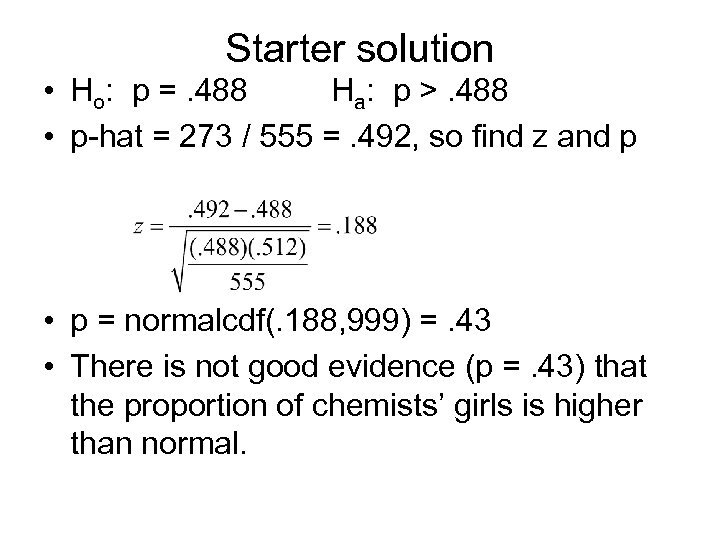Starter solution • Ho: p =. 488 Ha: p >. 488 • p-hat = 273 / 555 =. 492, so find z and p • p = normalcdf(. 188, 999) =. 43 • There is not good evidence (p =. 43) that the proportion of chemists’ girls is higher than normal.

Starter 12. 2. 1 One-sample procedures for proportions can also be used in matched pairs experiments. Here is an example: Each of 50 randomly selected subjects tastes two unmarked cups of coffee and says which he/she prefers. One cup in each pair contains instant coffee; the other is freshbrewed. 31 of the subjects prefer fresh-brewed. 1. 2. 3. Test the claim that a majority of people prefer the taste of fresh-brewed coffee. State hypotheses, check assumptions, find the test statistic and p-value. Is your result significant at the 5% level? Find a 90% confidence interval for the true proportion that prefer fresh-brewed. When you do an experiment like this, in what order should you present the two cups of coffee to the subjects?

Starter Solution • Ho: p =. 5 • Assumptions Ha: p >. 5 – SRS? OK – Large population? All coffee drinkers > 10 x 50 OK – At least 10 in each group? 50 x. 5 > 10 OK • z = 1. 70 p =. 045 • There is sufficient evidence (p<. 05) to support the claim that coffee drinkers prefer freshbrewed. • C. I. =. 62 ± 1. 645 x. 0686 = (. 507, . 733) • Randomization is needed in any experiment; flip a coin (or use another method) to choose which coffee each subject gets first. • See question on next slide:

The Cola Challenge! • Do Northgate students prefer Pepsi over Coke? In a randomized matched-pairs experiment we did last fall, here were the results: – Preferred Pepsi: 58 – Preferred Coke: 31 • Perform a hypothesis test of the claim that Pepsi is preferred.

Starter 12. 2. 2 The drug AZT is used to treat symptoms of AIDS. It was studied in an experiment involving volunteers already diagnosed as having HIV, the virus that causes AIDS. 435 subjects took AZT and another 435 took a placebo. At the end of the study, 17 of the AZT subjects had developed AIDS; 38 of the placebo subjects had developed AIDS. We want to test the claim that taking AZT lowers the proportion of people who go from HIV to AIDS. 1. 2. 3. 4. Assign numbers to the groups Verify that assumptions are met and state hypotheses Carry out the test on calculator and write your conclusion This experiment was double-blind. What does that mean?

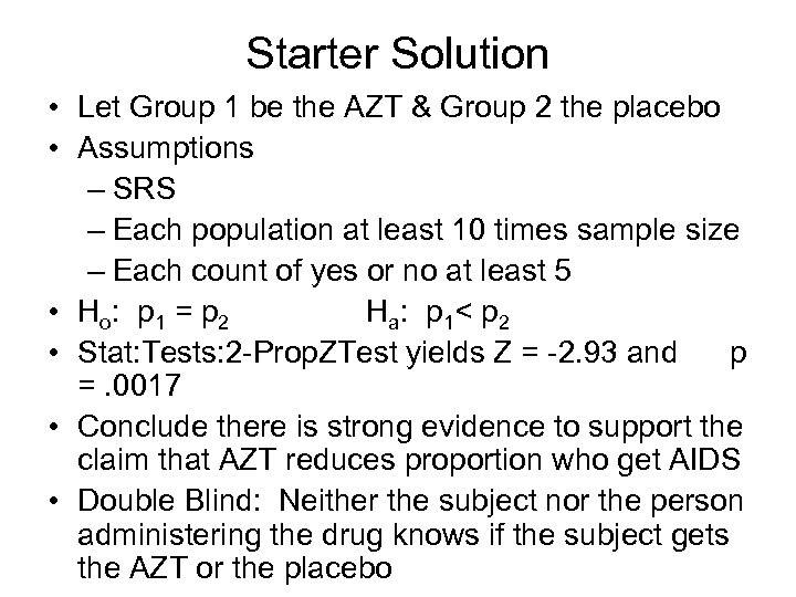Starter Solution • Let Group 1 be the AZT & Group 2 the placebo • Assumptions – SRS – Each population at least 10 times sample size – Each count of yes or no at least 5 • H o: p 1 = p 2 H a: p 1< p 2 • Stat: Tests: 2 -Prop. ZTest yields Z = -2. 93 and p =. 0017 • Conclude there is strong evidence to support the claim that AZT reduces proportion who get AIDS • Double Blind: Neither the subject nor the person administering the drug knows if the subject gets the AZT or the placebo

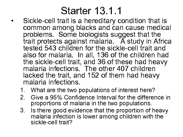Starter 13. 1. 1 • Sickle-cell trait is a hereditary condition that is common among blacks and can cause medical problems. Some biologists suggest that the trait protects against malaria. A study in Africa tested 543 children for the sickle-cell trait and also for malaria. In all, 136 of the children had the sickle-cell trait, and 36 of these had heavy malaria infections. The other 407 children lacked the trait, and 152 of them had heavy malaria infections. 1. What are the two populations of interest here? 2. Give a 95% Confidence Interval for the difference in proportions of malaria in the two populations. 3. Is there good evidence that the proportion of heavy malaria infection is lower among children with the sickle-cell trait?

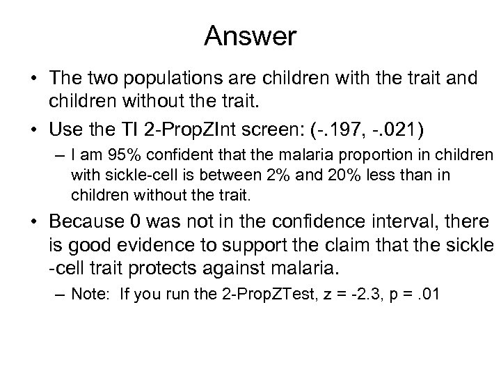Answer • The two populations are children with the trait and children without the trait. • Use the TI 2 -Prop. ZInt screen: (-. 197, -. 021) – I am 95% confident that the malaria proportion in children with sickle-cell is between 2% and 20% less than in children without the trait. • Because 0 was not in the confidence interval, there is good evidence to support the claim that the sickle -cell trait protects against malaria. – Note: If you run the 2 -Prop. ZTest, z = -2. 3, p =. 01

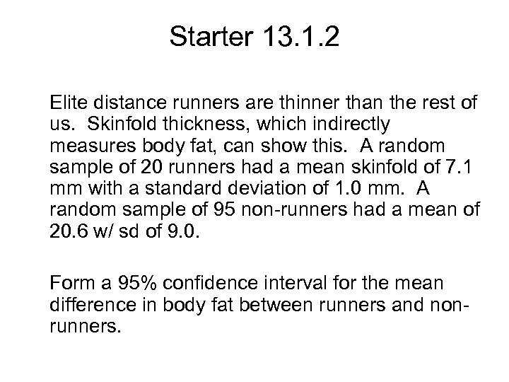Starter 13. 1. 2 Elite distance runners are thinner than the rest of us. Skinfold thickness, which indirectly measures body fat, can show this. A random sample of 20 runners had a mean skinfold of 7. 1 mm with a standard deviation of 1. 0 mm. A random sample of 95 non-runners had a mean of 20. 6 w/ sd of 9. 0. Form a 95% confidence interval for the mean difference in body fat between runners and nonrunners.

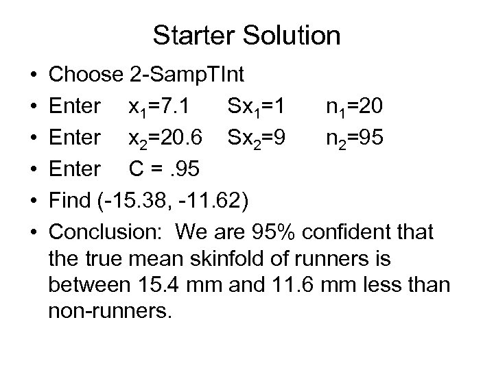Starter Solution • • • Choose 2 -Samp. TInt Enter x 1=7. 1 Sx 1=1 n 1=20 Enter x 2=20. 6 Sx 2=9 n 2=95 Enter C =. 95 Find (-15. 38, -11. 62) Conclusion: We are 95% confident that the true mean skinfold of runners is between 15. 4 mm and 11. 6 mm less than non-runners.

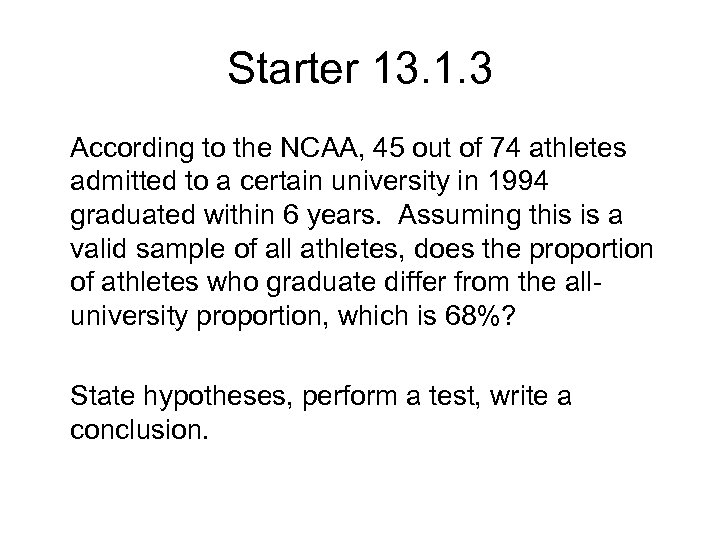Starter 13. 1. 3 According to the NCAA, 45 out of 74 athletes admitted to a certain university in 1994 graduated within 6 years. Assuming this is a valid sample of all athletes, does the proportion of athletes who graduate differ from the alluniversity proportion, which is 68%? State hypotheses, perform a test, write a conclusion.

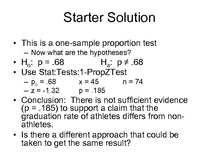Starter Solution • This is a one-sample proportion test – Now what are the hypotheses? • Ho: p =. 68 Ha: p ≠. 68 • Use Stat: Tests: 1 -Prop. ZTest – po =. 68 – z = -1. 32 x = 45 p =. 185 n = 74 • Conclusion: There is not sufficient evidence (p =. 185) to support a claim that the graduation rate of athletes differs from nonathletes. • Is there a different approach that could be taken to get the same result?

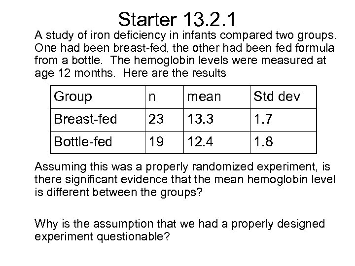Starter 13. 2. 1 A study of iron deficiency in infants compared two groups. One had been breast-fed, the other had been fed formula from a bottle. The hemoglobin levels were measured at age 12 months. Here are the results Group n mean Std dev Breast-fed 23 13. 3 1. 7 Bottle-fed 19 12. 4 1. 8 Assuming this was a properly randomized experiment, is there significant evidence that the mean hemoglobin level is different between the groups? Why is the assumption that we had a properly designed experiment questionable?

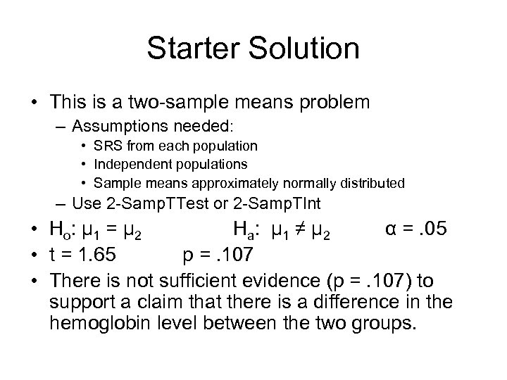Starter Solution • This is a two-sample means problem – Assumptions needed: • SRS from each population • Independent populations • Sample means approximately normally distributed – Use 2 -Samp. TTest or 2 -Samp. TInt • H o: μ 1 = μ 2 H a: μ 1 ≠ μ 2 α =. 05 • t = 1. 65 p =. 107 • There is not sufficient evidence (p =. 107) to support a claim that there is a difference in the hemoglobin level between the two groups.

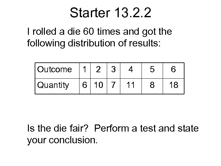Starter 13. 2. 2 I rolled a die 60 times and got the following distribution of results: Outcome 1 2 3 4 5 6 Quantity 6 10 7 11 8 18 Is the die fair? Perform a test and state your conclusion.

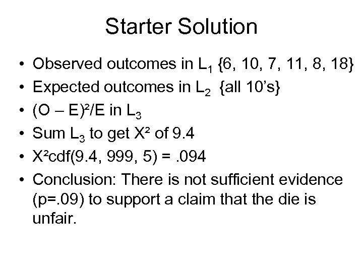Starter Solution • • • Observed outcomes in L 1 {6, 10, 7, 11, 8, 18} Expected outcomes in L 2 {all 10’s} (O – E)²/E in L 3 Sum L 3 to get X² of 9. 4 X²cdf(9. 4, 999, 5) =. 094 Conclusion: There is not sufficient evidence (p=. 09) to support a claim that the die is unfair.

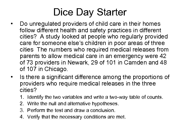Dice Day Starter • • Do unregulated providers of child care in their homes follow different health and safety practices in different cities? A study looked at people who regularly provided care for someone else’s children in poor areas of three cities The numbers who required medical releases from parents to allow medical care in an emergency were 42 of 73 providers in Newark, 29 of 101 in Camden and 48 of 107 in Chicago. Is there a significant difference among the proportions of providers who require medical releases in the three cities? 1. 2. 3. 4. Identify the two variables and write a two-way table of counts. Write the null and alternative hypotheses. Perform the test and draw a conclusion. Verify that the necessary conditions are met.

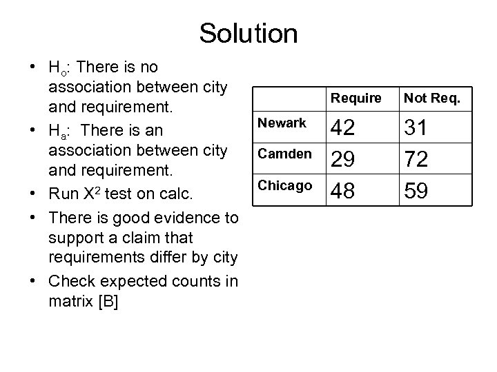Solution • Ho: There is no association between city and requirement. • Ha: There is an association between city and requirement. • Run X 2 test on calc. • There is good evidence to support a claim that requirements differ by city • Check expected counts in matrix [B] Require Newark Camden Chicago Not Req. 42 29 48 31 72 59

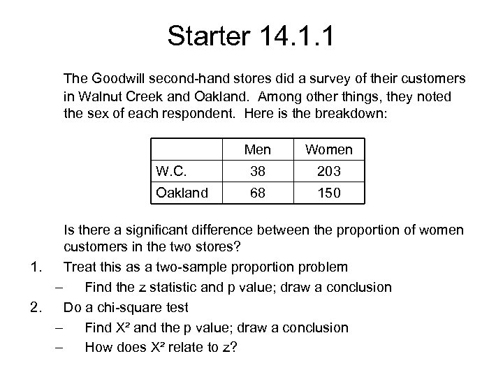Starter 14. 1. 1 The Goodwill second-hand stores did a survey of their customers in Walnut Creek and Oakland. Among other things, they noted the sex of each respondent. Here is the breakdown: Men Women W. C. 38 203 Oakland 68 150 Is there a significant difference between the proportion of women customers in the two stores? 1. Treat this as a two-sample proportion problem – Find the z statistic and p value; draw a conclusion 2. Do a chi-square test – Find X² and the p value; draw a conclusion – How does X² relate to z?

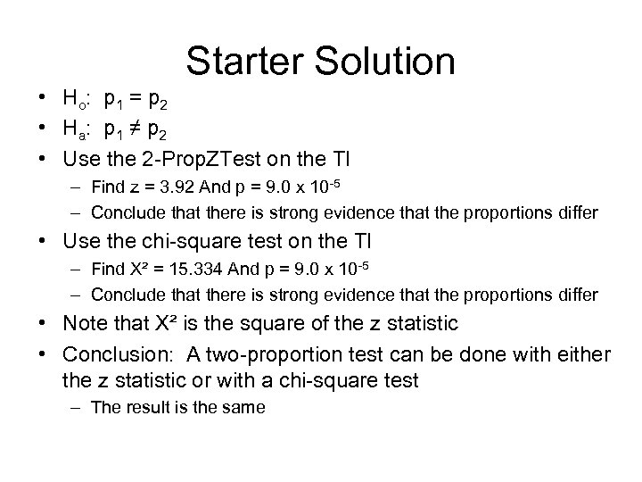Starter Solution • H o: p 1 = p 2 • H a: p 1 ≠ p 2 • Use the 2 -Prop. ZTest on the TI – Find z = 3. 92 And p = 9. 0 x 10 -5 – Conclude that there is strong evidence that the proportions differ • Use the chi-square test on the TI – Find X² = 15. 334 And p = 9. 0 x 10 -5 – Conclude that there is strong evidence that the proportions differ • Note that X² is the square of the z statistic • Conclusion: A two-proportion test can be done with either the z statistic or with a chi-square test – The result is the same

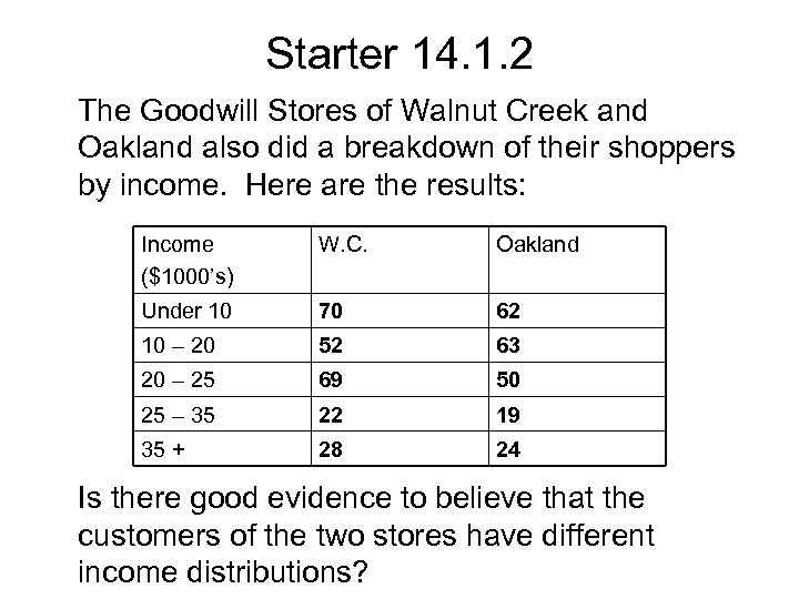Starter 14. 1. 2 The Goodwill Stores of Walnut Creek and Oakland also did a breakdown of their shoppers by income. Here are the results: Income ($1000’s) W. C. Oakland Under 10 70 62 10 – 20 52 63 20 – 25 69 50 25 – 35 22 19 35 + 28 24 Is there good evidence to believe that the customers of the two stores have different income distributions?

Starter Solution • Ho: There is no difference in the income distributions • Ha: The income distributions differ • Put the two-way table into matrix [A] • Run the chi-square Test • X 2 = 3. 955 p =. 412 • Conclusion: There is not sufficient evidence (p =. 412) to support a claim that the income distributions are different

Starter 14. 3. 1 Men and women were observed playing a game of chance. 3 of 12 men won the game; 8 of 12 women won. Is there a statistically significant difference between the men’s and women’s results? State hypotheses, perform a test and write a conclusion

Starter solution • This asks for a comparison of proportions from two populations • Use 2 -Prop. ZTest screen – Choose p 1 ≠ p 2 alternative – Get z = 2. 05 and p = 0. 04 • Or use X 2 Test screen – Get X 2 = 4. 196 and p =. 04 • Conclusion: – There is good evidence (p =. 04) that the winning proportions are different for men and women – Checking matrix [B] shows all expected counts are at least 5.