6dbbaa849bb88f54314238f0d150d5b3.ppt
- Количество слайдов: 139
 Unit-4 © 2014 Pearson Education, Inc. 12 - 1
 Inventory Management © 2014 Pearson Education, Inc. 12 12 - 2
 Outline ► ► ► Global Company Profile: Amazon. com The Importance of Inventory Managing Inventory Models for Independent Demand © 2014 Pearson Education, Inc. 12 - 3
 Outline - Continued ► ► ► Probabilistic Models and Safety Stock Single-Period Model Fixed-Period (P) Systems © 2014 Pearson Education, Inc. 12 - 4
 Learning Objectives When you complete this chapter you should be able to: 1. Conduct an ABC analysis 2. Explain and use cycle counting 3. Explain and use the EOQ model for independent inventory demand 4. Compute a reorder point and safety stock © 2014 Pearson Education, Inc. 12 - 5
 Learning Objectives When you complete this chapter you should be able to: 5. Apply the production order quantity model 6. Explain and use the quantity discount model 7. Understand service levels and probabilistic inventory models © 2014 Pearson Education, Inc. 12 - 6
 Inventory Management at Amazon. com ► ► Amazon. com started as a “virtual” retailer – no inventory, no warehouses, no overhead; just computers taking orders to be filled by others Growth has forced Amazon. com to become a world leader in warehousing and inventory management © 2014 Pearson Education, Inc. © 2014 Pearson Education, 12 - 7
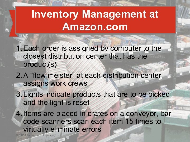 Inventory Management at Amazon. com 1. Each order is assigned by computer to the closest distribution center that has the product(s) 2. A “flow meister” at each distribution center assigns work crews 3. Lights indicate products that are to be picked and the light is reset 4. Items are placed in crates on a conveyor, bar code scanners scan each item 15 times to virtually eliminate errors © 2014 Pearson Education, Inc. © 2014 Pearson Education, 12 - 8
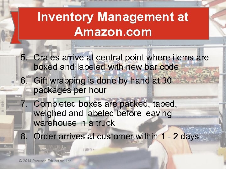 Inventory Management at Amazon. com 5. Crates arrive at central point where items are boxed and labeled with new bar code 6. Gift wrapping is done by hand at 30 packages per hour 7. Completed boxes are packed, taped, weighed and labeled before leaving warehouse in a truck 8. Order arrives at customer within 1 - 2 days © 2014 Pearson Education, Inc. © 2014 Pearson Education, 12 - 9
 Inventory Management The objective of inventory management is to strike a balance between inventory investment and customer service © 2014 Pearson Education, Inc. 12 - 10
 Importance of Inventory ▶ One of the most expensive assets of many companies representing as much as 50% of total invested capital ▶ Operations managers must balance inventory investment and customer service © 2014 Pearson Education, Inc. 12 - 11
 Functions of Inventory 1. To provide a selection of goods for anticipated demand to separate the firm from fluctuations in demand 2. To decouple or separate various parts of the production process 3. To take advantage of quantity discounts 4. To hedge against inflation © 2014 Pearson Education, Inc. 12 - 12
 Types of Inventory ▶ Raw material ▶ Purchased but not processed ▶ Work-in-process (WIP) ▶ Undergone some change but not completed ▶ A function of cycle time for a product ▶ Maintenance/repair/operating (MRO) ▶ Necessary to keep machinery and processes productive ▶ Finished goods ▶ Completed product awaiting shipment © 2014 Pearson Education, Inc. 12 - 13
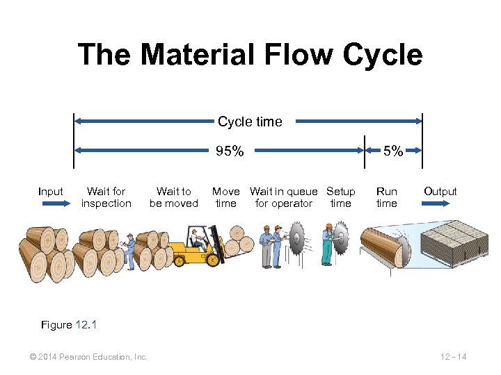 The Material Flow Cycle time 95% Input Wait for inspection Wait to be moved Move Wait in queue Setup time for operator time 5% Run time Output Figure 12. 1 © 2014 Pearson Education, Inc. 12 - 14
 Managing Inventory 1. How inventory items can be classified (ABC analysis) 2. How accurate inventory records can be maintained © 2014 Pearson Education, Inc. 12 - 15
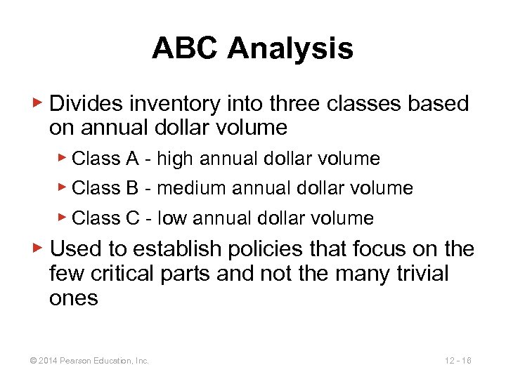 ABC Analysis ▶ Divides inventory into three classes based on annual dollar volume ▶ Class A - high annual dollar volume ▶ Class B - medium annual dollar volume ▶ Class C - low annual dollar volume ▶ Used to establish policies that focus on the few critical parts and not the many trivial ones © 2014 Pearson Education, Inc. 12 - 16
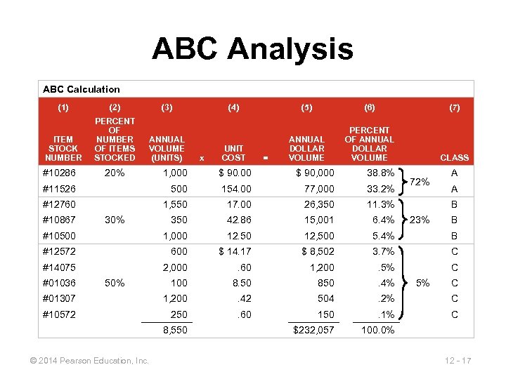 ABC Analysis ABC Calculation (1) (2) (3) ITEM STOCK NUMBER PERCENT OF NUMBER OF ITEMS STOCKED ANNUAL VOLUME (UNITS) #10286 x (5) (6) (7) UNIT COST ANNUAL DOLLAR VOLUME PERCENT OF ANNUAL DOLLAR VOLUME CLASS = 1, 000 $ 90, 000 38. 8% #11526 500 154. 00 77, 000 33. 2% #12760 1, 550 17. 00 26, 350 11. 3% 350 42. 86 15, 001 6. 4% #10500 1, 000 12. 50 12, 500 5. 4% B #12572 600 $ 14. 17 $ 8, 502 3. 7% C #14075 2, 000 . 60 1, 200 . 5% C 100 8. 50 850 . 4% #01307 1, 200 . 42 504 . 2% C #10572 250 . 60 150 . 1% C $232, 057 100. 0% #10867 #01036 20% (4) 30% 50% 8, 550 © 2014 Pearson Education, Inc. 72% A A B 23% 5% B C 12 - 17
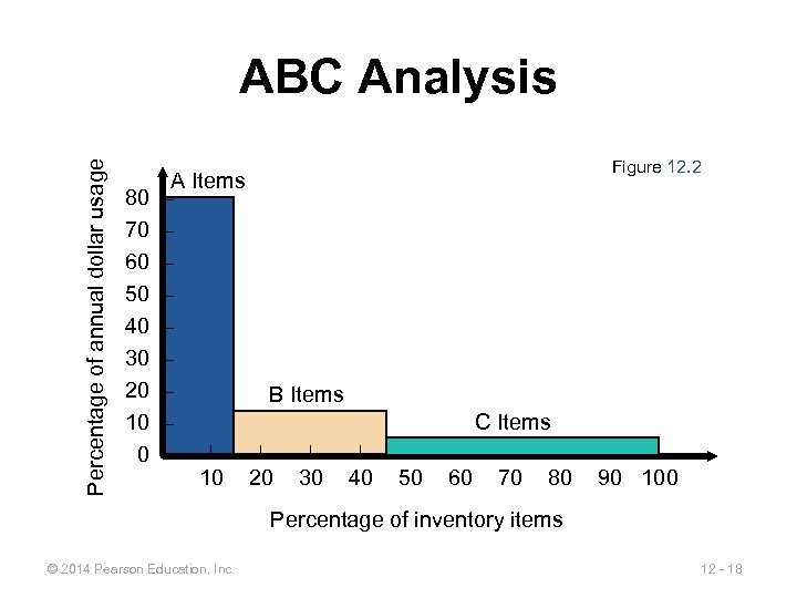 Percentage of annual dollar usage ABC Analysis 80 70 60 50 40 30 20 10 0 A Items – – – – B Items – | | – 10 20 30 40 Figure 12. 2 C Items | | 50 60 70 80 | | 90 100 Percentage of inventory items © 2014 Pearson Education, Inc. 12 - 18
 ABC Analysis ▶ Other criteria than annual dollar volume may be used ▶ ▶ High shortage or holding cost Anticipated engineering changes Delivery problems Quality problems © 2014 Pearson Education, Inc. 12 - 19
 ABC Analysis ▶ Policies employed may include 1. More emphasis on supplier development for A items 2. Tighter physical inventory control for A items 3. More care in forecasting A items © 2014 Pearson Education, Inc. 12 - 20
 Record Accuracy ► Accurate records are a critical ingredient in production and inventory systems ► Periodic systems require regular checks of inventory ► ► Two-bin system Perpetual inventory tracks receipts and subtractions on a continuing basis ► May be semi-automated © 2014 Pearson Education, Inc. 12 - 21
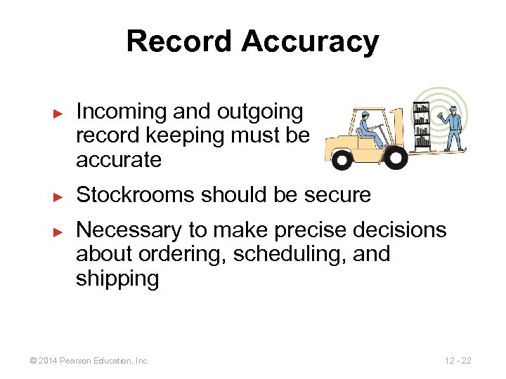 Record Accuracy ► ► ► Incoming and outgoing record keeping must be accurate Stockrooms should be secure Necessary to make precise decisions about ordering, scheduling, and shipping © 2014 Pearson Education, Inc. 12 - 22
 Cycle Counting ▶ Items are counted and records updated on a periodic basis ▶ Often used with ABC analysis ▶ Has several advantages 1. 2. 3. 4. Eliminates shutdowns and interruptions Eliminates annual inventory adjustment Trained personnel audit inventory accuracy Allows causes of errors to be identified and corrected 5. Maintains accurate inventory records © 2014 Pearson Education, Inc. 12 - 23
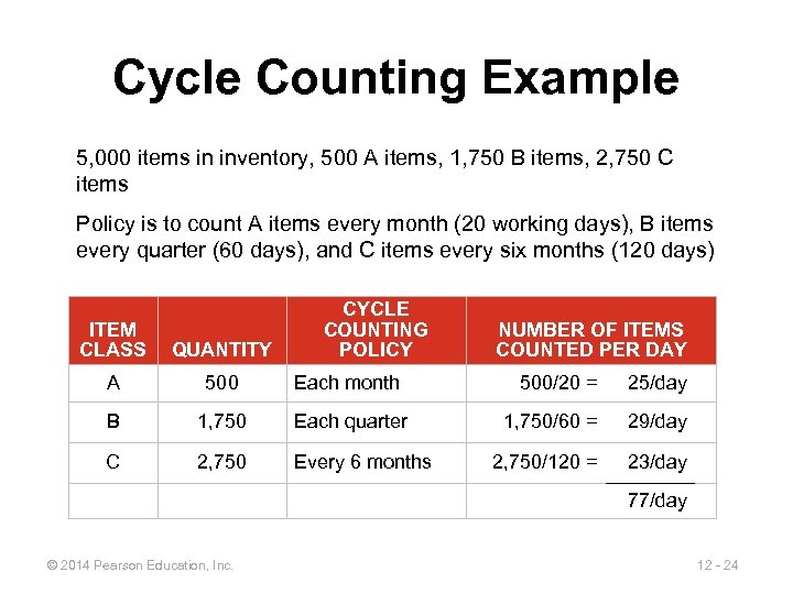 Cycle Counting Example 5, 000 items in inventory, 500 A items, 1, 750 B items, 2, 750 C items Policy is to count A items every month (20 working days), B items every quarter (60 days), and C items every six months (120 days) CYCLE COUNTING POLICY ITEM CLASS QUANTITY A 500 Each month B 1, 750 Each quarter C 2, 750 Every 6 months NUMBER OF ITEMS COUNTED PER DAY 500/20 = 25/day 1, 750/60 = 29/day 2, 750/120 = 23/day 77/day © 2014 Pearson Education, Inc. 12 - 24
 Control of Service Inventories ▶ Can be a critical component of profitability ▶ Losses may come from shrinkage or pilferage ▶ Applicable techniques include 1. Good personnel selection, training, and discipline 2. Tight control of incoming shipments 3. Effective control of all goods leaving facility © 2014 Pearson Education, Inc. 12 - 25
 Inventory Models ▶ Independent demand - the demand for item is independent of the demand for any other item in inventory ▶ Dependent demand - the demand for item is dependent upon the demand for some other item in the inventory © 2014 Pearson Education, Inc. 12 - 26
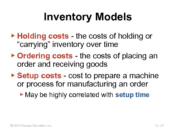 Inventory Models ▶ Holding costs - the costs of holding or “carrying” inventory over time ▶ Ordering costs - the costs of placing an order and receiving goods ▶ Setup costs - cost to prepare a machine or process for manufacturing an order ▶ May be highly correlated with setup time © 2014 Pearson Education, Inc. 12 - 27
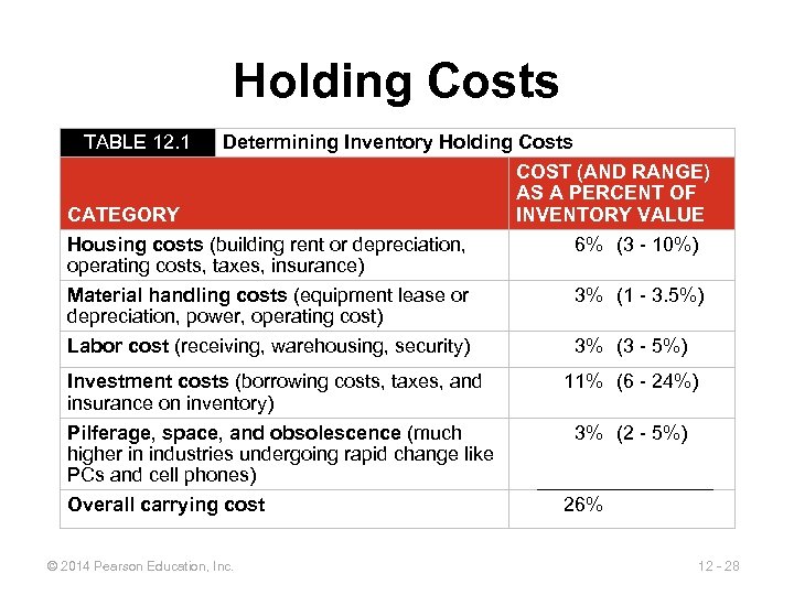 Holding Costs TABLE 12. 1 Determining Inventory Holding Costs COST (AND RANGE) AS A PERCENT OF CATEGORY INVENTORY VALUE Housing costs (building rent or depreciation, 6% (3 - 10%) operating costs, taxes, insurance) Material handling costs (equipment lease or 3% (1 - 3. 5%) depreciation, power, operating cost) Labor cost (receiving, warehousing, security) 3% (3 - 5%) Investment costs (borrowing costs, taxes, and insurance on inventory) Pilferage, space, and obsolescence (much higher in industries undergoing rapid change like PCs and cell phones) Overall carrying cost © 2014 Pearson Education, Inc. 11% (6 - 24%) 3% (2 - 5%) 26% 12 - 28
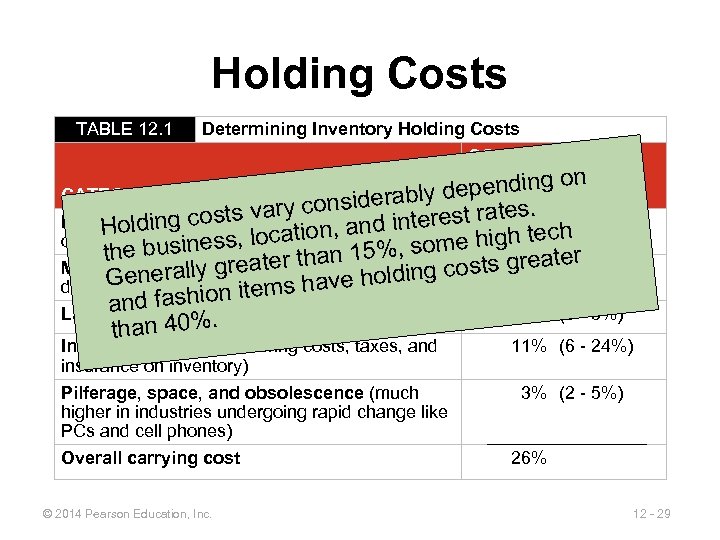 Holding Costs TABLE 12. 1 Determining Inventory Holding Costs COST (AND RANGE) AS A PERCENT OF pending on de. INVENTORY VALUE CATEGORY bly y considera erest rates. ar Housinglding costs v rent or depreciation, costs (building 6% (3 - 10%) Ho ion, and int me high tech at operating costs, ness, insurance) usi taxes, loc than 15%, so the b er Material handling costs t(equipment lease iorg costs great(1 - 3. 5%) 3% grea er ally Generpower, operatinghave hold n depreciation, s cost) fashion item nd Labora cost (receiving, warehousing, security) 3% (3 - 5%). than 40% Investment costs (borrowing costs, taxes, and insurance on inventory) Pilferage, space, and obsolescence (much higher in industries undergoing rapid change like PCs and cell phones) Overall carrying cost © 2014 Pearson Education, Inc. 11% (6 - 24%) 3% (2 - 5%) 26% 12 - 29
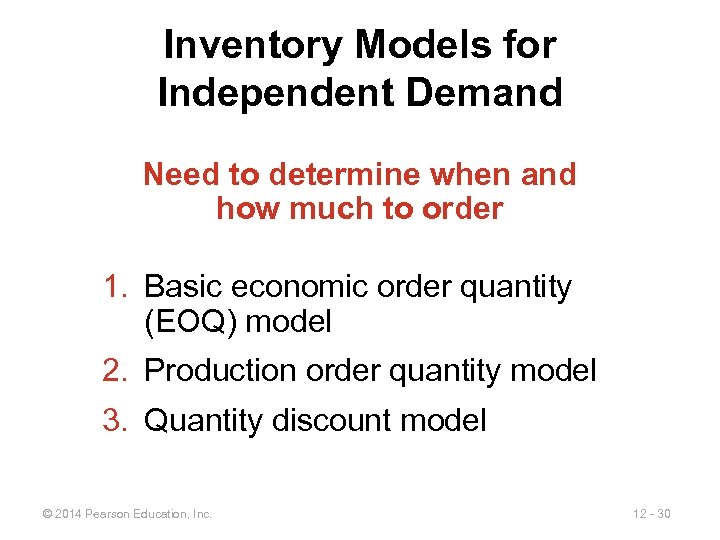 Inventory Models for Independent Demand Need to determine when and how much to order 1. Basic economic order quantity (EOQ) model 2. Production order quantity model 3. Quantity discount model © 2014 Pearson Education, Inc. 12 - 30
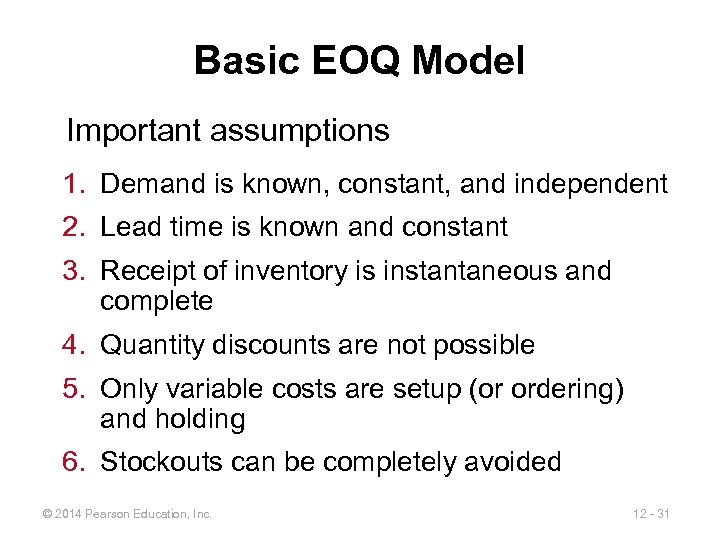 Basic EOQ Model Important assumptions 1. Demand is known, constant, and independent 2. Lead time is known and constant 3. Receipt of inventory is instantaneous and complete 4. Quantity discounts are not possible 5. Only variable costs are setup (or ordering) and holding 6. Stockouts can be completely avoided © 2014 Pearson Education, Inc. 12 - 31
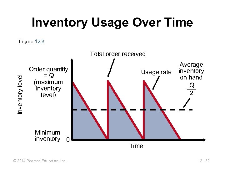 Inventory Usage Over Time Figure 12. 3 Inventory level Total order received Order quantity =Q (maximum inventory level) Minimum inventory 0 © 2014 Pearson Education, Inc. Usage rate Average inventory on hand Q 2 Time 12 - 32
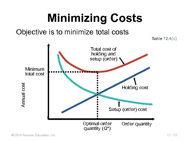 Minimizing Costs Objective is to minimize total costs Table 12. 4(c) Total cost of holding and setup (order) Annual cost Minimum total cost Holding cost Setup (order) cost Optimal order quantity (Q*) © 2014 Pearson Education, Inc. Order quantity 12 - 33
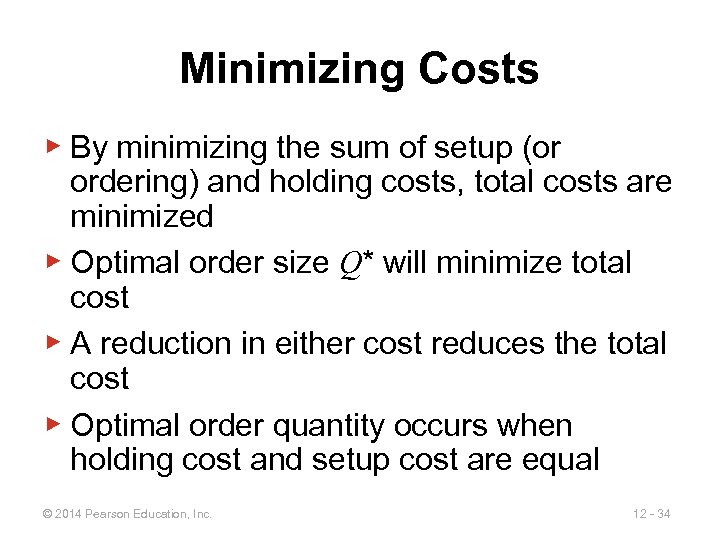 Minimizing Costs ▶ By minimizing the sum of setup (or ordering) and holding costs, total costs are minimized ▶ Optimal order size Q* will minimize total cost ▶ A reduction in either cost reduces the total cost ▶ Optimal order quantity occurs when holding cost and setup cost are equal © 2014 Pearson Education, Inc. 12 - 34
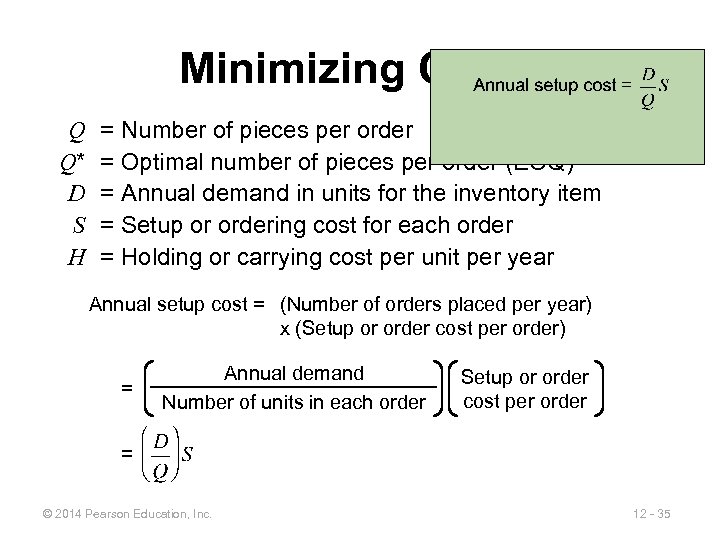 Minimizing Costs Q Q* D S H = Number of pieces per order = Optimal number of pieces per order (EOQ) = Annual demand in units for the inventory item = Setup or ordering cost for each order = Holding or carrying cost per unit per year Annual setup cost = (Number of orders placed per year) x (Setup or order cost per order) = Annual demand Number of units in each order © 2014 Pearson Education, Inc. Setup or order cost per order 12 - 35
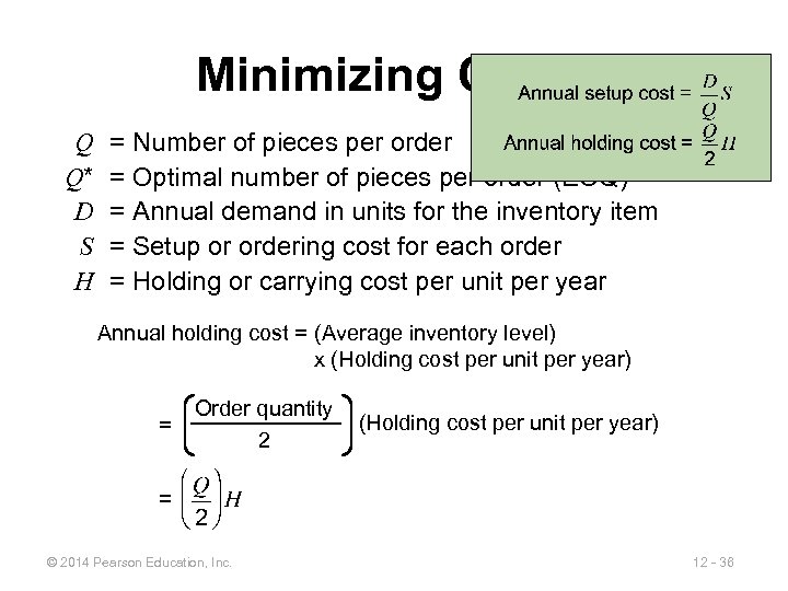 Minimizing Costs Q Q* D S H = Number of pieces per order = Optimal number of pieces per order (EOQ) = Annual demand in units for the inventory item = Setup or ordering cost for each order = Holding or carrying cost per unit per year Annual holding cost = (Average inventory level) x (Holding cost per unit per year) = Order quantity 2 © 2014 Pearson Education, Inc. (Holding cost per unit per year) 12 - 36
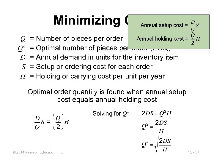 Minimizing Costs Q Q* D S H = Number of pieces per order = Optimal number of pieces per order (EOQ) = Annual demand in units for the inventory item = Setup or ordering cost for each order = Holding or carrying cost per unit per year Optimal order quantity is found when annual setup cost equals annual holding cost Solving for Q* © 2014 Pearson Education, Inc. 12 - 37
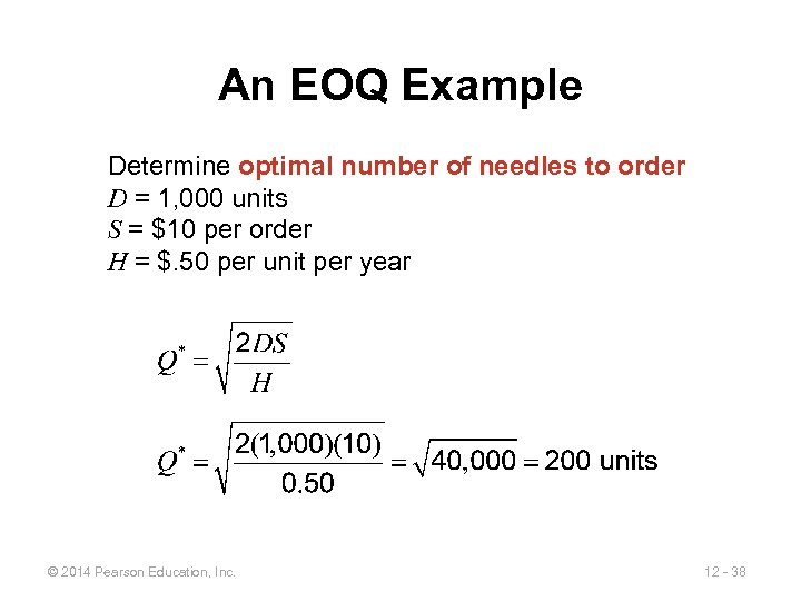 An EOQ Example Determine optimal number of needles to order D = 1, 000 units S = $10 per order H = $. 50 per unit per year © 2014 Pearson Education, Inc. 12 - 38
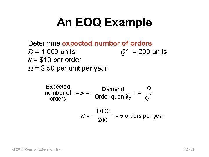 An EOQ Example Determine expected number of orders D = 1, 000 units Q* = 200 units S = $10 per order H = $. 50 per unit per year Expected Demand number of = N = Order quantity orders = 1, 000 N= = 5 orders per year 200 © 2014 Pearson Education, Inc. 12 - 39
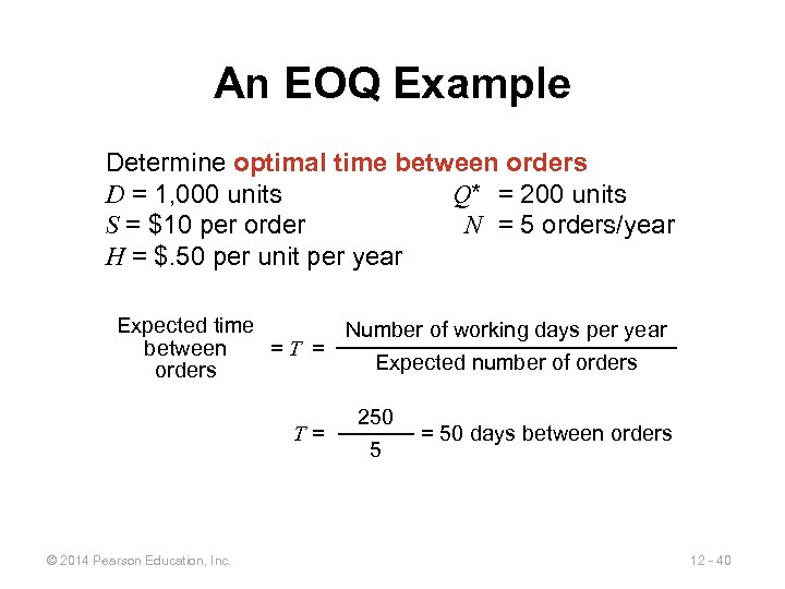 An EOQ Example Determine optimal time between orders D = 1, 000 units Q* = 200 units S = $10 per order N = 5 orders/year H = $. 50 per unit per year Expected time Number of working days per year between =T = Expected number of orders T= © 2014 Pearson Education, Inc. 250 5 = 50 days between orders 12 - 40
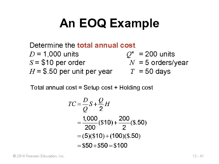 An EOQ Example Determine the total annual cost D = 1, 000 units Q* = 200 units S = $10 per order N = 5 orders/year H = $. 50 per unit per year T = 50 days Total annual cost = Setup cost + Holding cost © 2014 Pearson Education, Inc. 12 - 41
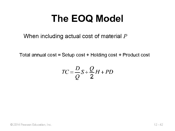 The EOQ Model When including actual cost of material P Total annual cost = Setup cost + Holding cost + Product cost © 2014 Pearson Education, Inc. 12 - 42
 Robust Model ▶ The EOQ model is robust ▶ It works even if all parameters and assumptions are not met ▶ The total cost curve is relatively flat in the area of the EOQ © 2014 Pearson Education, Inc. 12 - 43
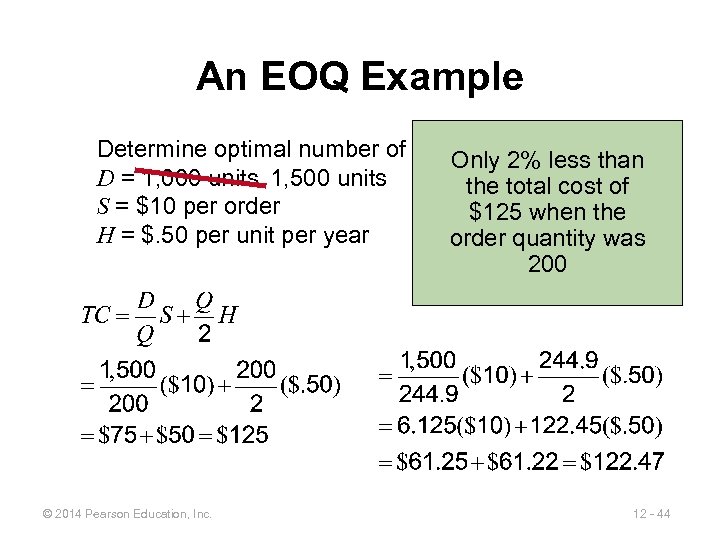 An EOQ Example Determine optimal number of needles to order than Only 2% less D = 1, 000 units 1, 500 units Q* =the total cost of 200 units S = $10 per order N =$125 when the 5 orders/year H = $. 50 per unit per year T order days = 50 quantity was 200 © 2014 Pearson Education, Inc. 12 - 44
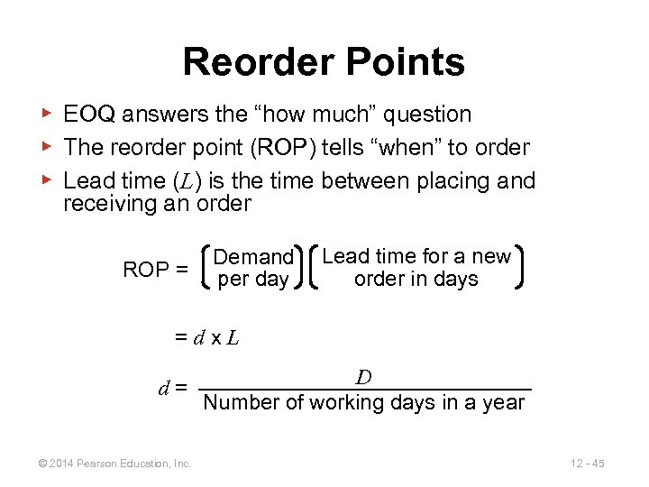 Reorder Points ▶ EOQ answers the “how much” question ▶ The reorder point (ROP) tells “when” to order ▶ Lead time (L) is the time between placing and receiving an order ROP = Demand per day Lead time for a new order in days =dx. L d= © 2014 Pearson Education, Inc. D Number of working days in a year 12 - 45
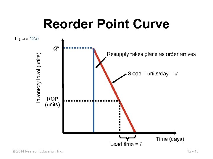 Reorder Point Curve Figure 12. 5 Inventory level (units) Q* Resupply takes place as order arrives Slope = units/day = d ROP (units) Lead time = L © 2014 Pearson Education, Inc. Time (days) 12 - 46
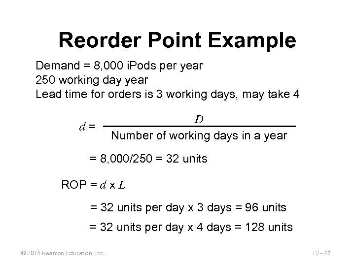 Reorder Point Example Demand = 8, 000 i. Pods per year 250 working day year Lead time for orders is 3 working days, may take 4 d= D Number of working days in a year = 8, 000/250 = 32 units ROP = d x L = 32 units per day x 3 days = 96 units = 32 units per day x 4 days = 128 units © 2014 Pearson Education, Inc. 12 - 47
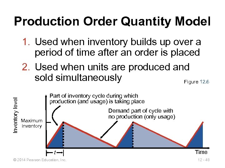 Production Order Quantity Model Inventory level 1. Used when inventory builds up over a period of time after an order is placed 2. Used when units are produced and sold simultaneously Figure 12. 6 Part of inventory cycle during which production (and usage) is taking place Demand part of cycle with no production (only usage) Maximum inventory t © 2014 Pearson Education, Inc. Time 12 - 48
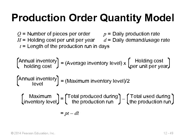 Production Order Quantity Model Q = Number of pieces per order p = Daily production rate H = Holding cost per unit per year d = Daily demand/usage rate t = Length of the production run in days Annual inventory = (Average inventory level) x Holding cost holding cost per unit per year Annual inventory = (Maximum inventory level)/2 level Maximum = Total produced during – Total used during inventory level the production run = pt – dt © 2014 Pearson Education, Inc. 12 - 49
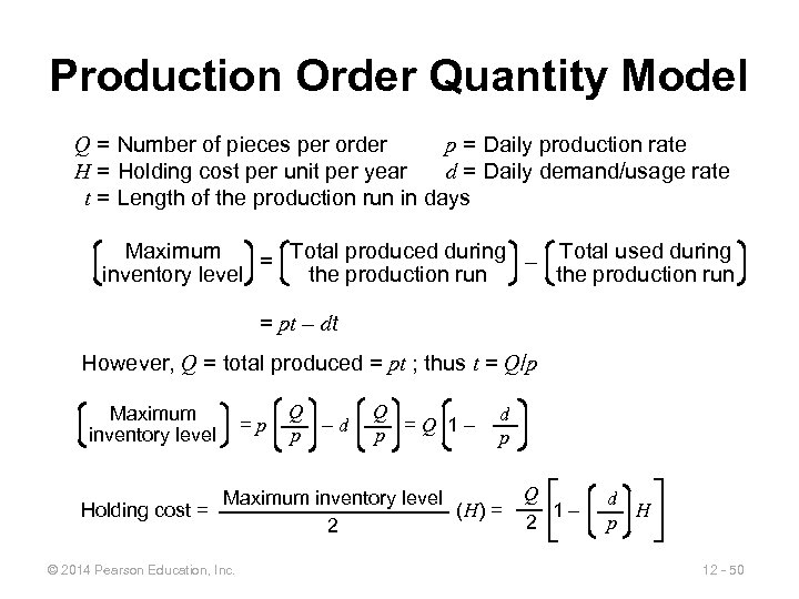 Production Order Quantity Model Q = Number of pieces per order p = Daily production rate H = Holding cost per unit per year d = Daily demand/usage rate t = Length of the production run in days Maximum = Total produced during – Total used during the production run inventory level the production run = pt – dt However, Q = total produced = pt ; thus t = Q/p Maximum inventory level =p Q p –d Q p =Q 1– d p Maximum inventory level Holding cost = (H) = 2 © 2014 Pearson Education, Inc. Q 1– 2 d H p 12 - 50
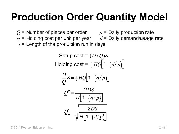 Production Order Quantity Model Q = Number of pieces per order p = Daily production rate H = Holding cost per unit per year d = Daily demand/usage rate t = Length of the production run in days © 2014 Pearson Education, Inc. 12 - 51
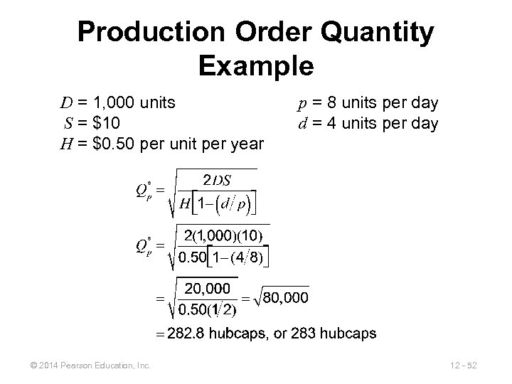 Production Order Quantity Example D = 1, 000 units S = $10 H = $0. 50 per unit per year © 2014 Pearson Education, Inc. p = 8 units per day d = 4 units per day 12 - 52
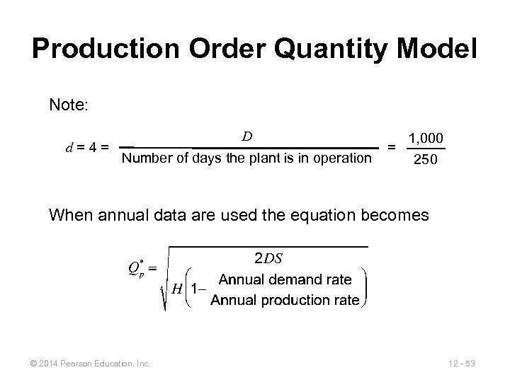 Production Order Quantity Model Note: d=4= D Number of days the plant is in operation = 1, 000 250 When annual data are used the equation becomes © 2014 Pearson Education, Inc. 12 - 53
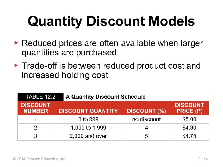 Quantity Discount Models ▶ Reduced prices are often available when larger quantities are purchased ▶ Trade-off is between reduced product cost and increased holding cost TABLE 12. 2 A Quantity Discount Schedule DISCOUNT NUMBER DISCOUNT QUANTITY DISCOUNT (%) 1 0 to 999 no discount 2 1, 000 to 1, 999 4 3 © 2014 Pearson Education, Inc. 2, 000 and over 5 DISCOUNT PRICE (P) $5. 00 $4. 80 $4. 75 12 - 54
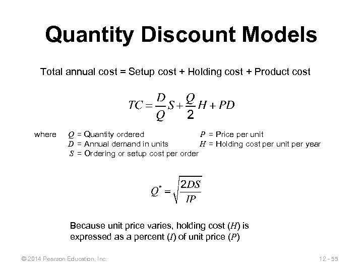 Quantity Discount Models Total annual cost = Setup cost + Holding cost + Product cost where Q = Quantity ordered P = Price per unit D = Annual demand in units H = Holding cost per unit per year S = Ordering or setup cost per order Because unit price varies, holding cost (H) is expressed as a percent (I) of unit price (P) © 2014 Pearson Education, Inc. 12 - 55
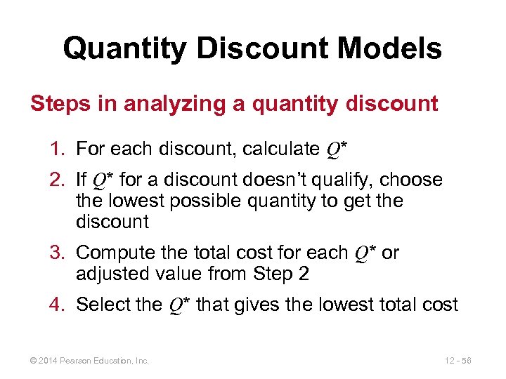 Quantity Discount Models Steps in analyzing a quantity discount 1. For each discount, calculate Q* 2. If Q* for a discount doesn’t qualify, choose the lowest possible quantity to get the discount 3. Compute the total cost for each Q* or adjusted value from Step 2 4. Select the Q* that gives the lowest total cost © 2014 Pearson Education, Inc. 12 - 56
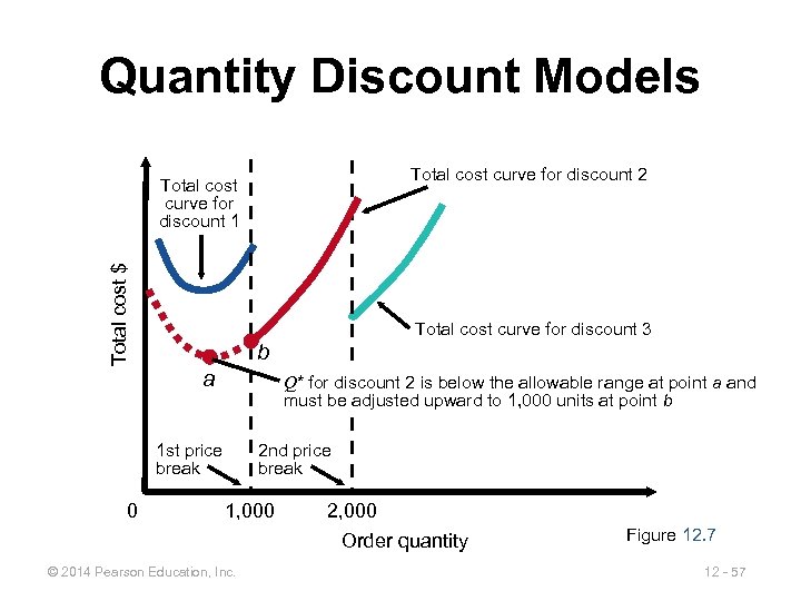 Quantity Discount Models Total cost curve for discount 2 Total cost $ Total cost curve for discount 1 Total cost curve for discount 3 b a Q* for discount 2 is below the allowable range at point a and must be adjusted upward to 1, 000 units at point b 1 st price break 0 2 nd price break 1, 000 2, 000 Order quantity © 2014 Pearson Education, Inc. Figure 12. 7 12 - 57
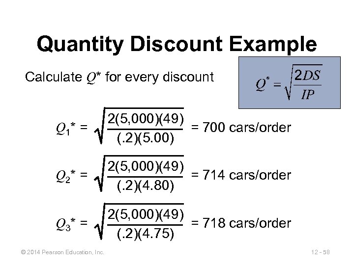 Quantity Discount Example Calculate Q* for every discount Q 1* = 2(5, 000)(49) = 700 cars/order (. 2)(5. 00) Q 2* = 2(5, 000)(49) = 714 cars/order (. 2)(4. 80) Q 3* = 2(5, 000)(49) = 718 cars/order (. 2)(4. 75) © 2014 Pearson Education, Inc. 12 - 58
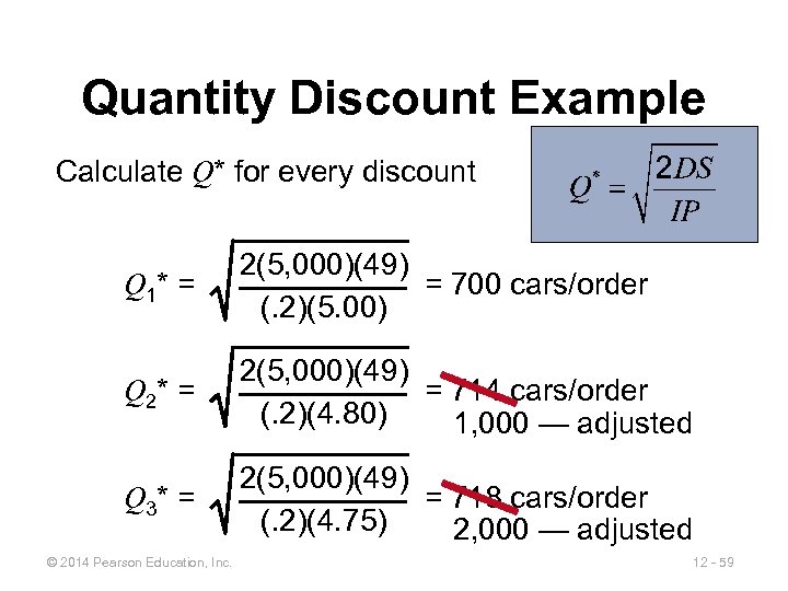 Quantity Discount Example Calculate Q* for every discount Q 1* = 2(5, 000)(49) = 700 cars/order (. 2)(5. 00) Q 2* = 2(5, 000)(49) = 714 cars/order (. 2)(4. 80) 1, 000 — adjusted Q 3* = 2(5, 000)(49) = 718 cars/order (. 2)(4. 75) 2, 000 — adjusted © 2014 Pearson Education, Inc. 12 - 59
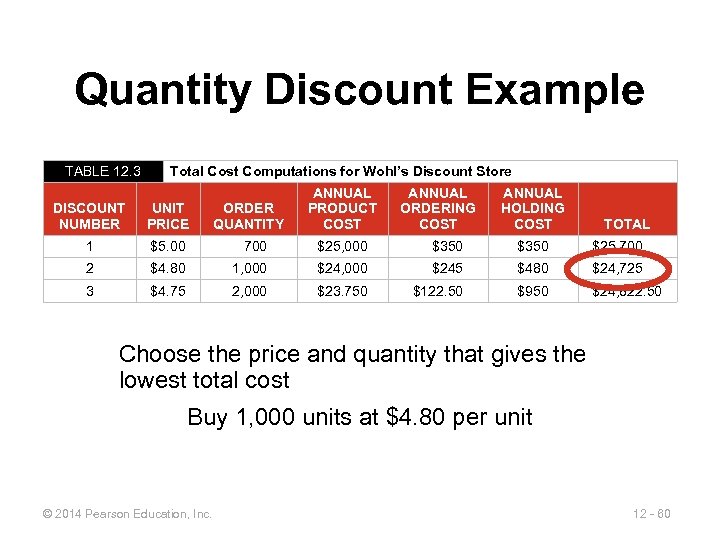 Quantity Discount Example TABLE 12. 3 Total Cost Computations for Wohl’s Discount Store ORDER QUANTITY ANNUAL PRODUCT COST ANNUAL ORDERING COST ANNUAL HOLDING COST DISCOUNT NUMBER UNIT PRICE 1 $5. 00 700 $25, 000 $350 $25, 700 2 $4. 80 1, 000 $245 $480 $24, 725 3 $4. 75 2, 000 $23. 750 $122. 50 $950 $24, 822. 50 TOTAL Choose the price and quantity that gives the lowest total cost Buy 1, 000 units at $4. 80 per unit © 2014 Pearson Education, Inc. 12 - 60
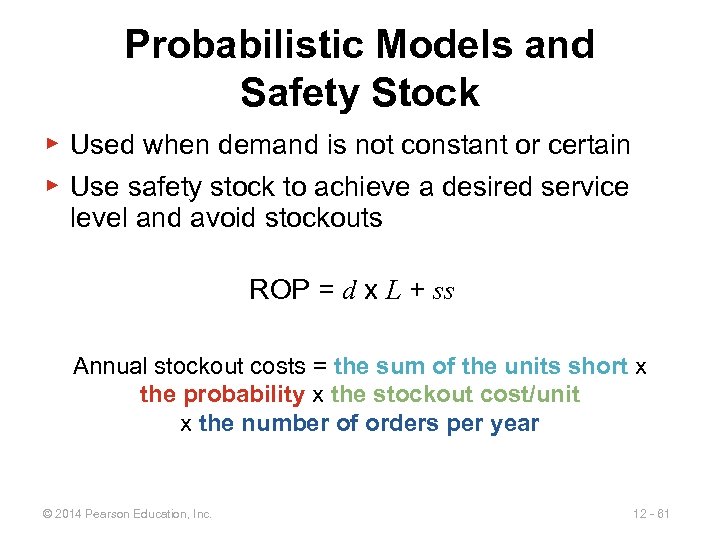 Probabilistic Models and Safety Stock ▶ Used when demand is not constant or certain ▶ Use safety stock to achieve a desired service level and avoid stockouts ROP = d x L + ss Annual stockout costs = the sum of the units short x the probability x the stockout cost/unit x the number of orders per year © 2014 Pearson Education, Inc. 12 - 61
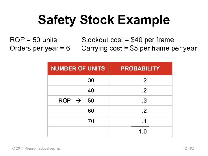 Safety Stock Example ROP = 50 units Orders per year = 6 Stockout cost = $40 per frame Carrying cost = $5 per frame per year NUMBER OF UNITS PROBABILITY 30 40 . 2 50 . 3 60 . 2 70 ROP . 2 . 1 1. 0 © 2014 Pearson Education, Inc. 12 - 62
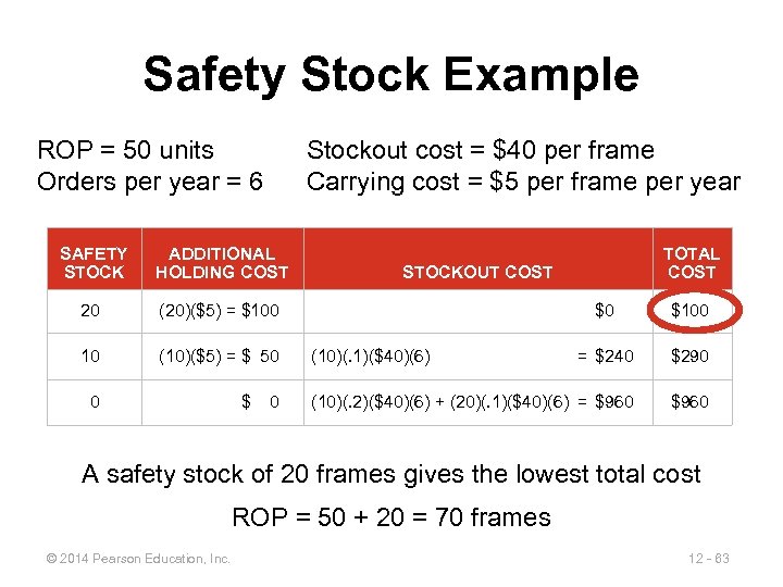 Safety Stock Example ROP = 50 units Orders per year = 6 Stockout cost = $40 per frame Carrying cost = $5 per frame per year SAFETY STOCK ADDITIONAL HOLDING COST 20 (20)($5) = $100 10 (10)($5) = $ 50 0 $ 0 TOTAL COST STOCKOUT COST $0 $100 = $240 $290 (10)(. 2)($40)(6) + (20)(. 1)($40)(6) = $960 (10)(. 1)($40)(6) A safety stock of 20 frames gives the lowest total cost ROP = 50 + 20 = 70 frames © 2014 Pearson Education, Inc. 12 - 63
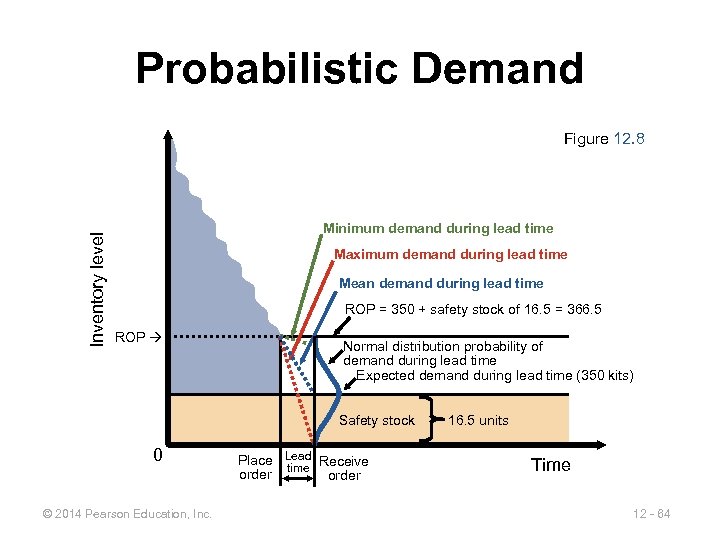 Probabilistic Demand Inventory level Figure 12. 8 Minimum demand during lead time Maximum demand during lead time Mean demand during lead time ROP = 350 + safety stock of 16. 5 = 366. 5 ROP Normal distribution probability of demand during lead time Expected demand during lead time (350 kits) Safety stock 0 © 2014 Pearson Education, Inc. Place Lead Receive time order 16. 5 units Time 12 - 64
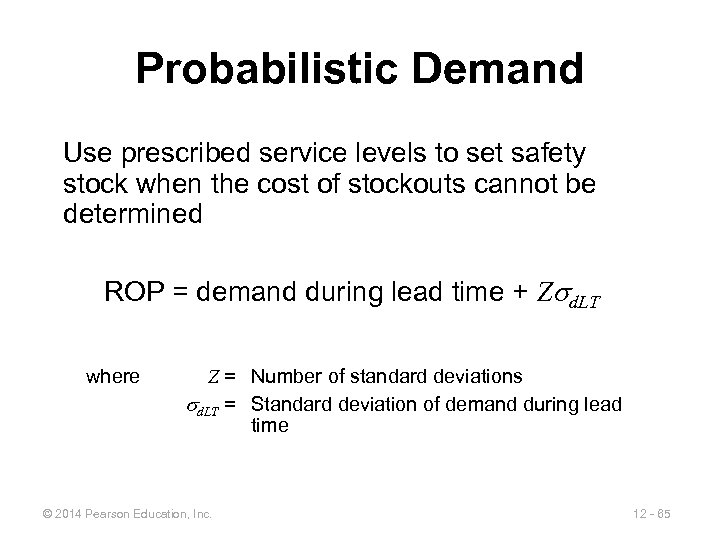 Probabilistic Demand Use prescribed service levels to set safety stock when the cost of stockouts cannot be determined ROP = demand during lead time + Z d. LT where Z = Number of standard deviations d. LT = Standard deviation of demand during lead time © 2014 Pearson Education, Inc. 12 - 65
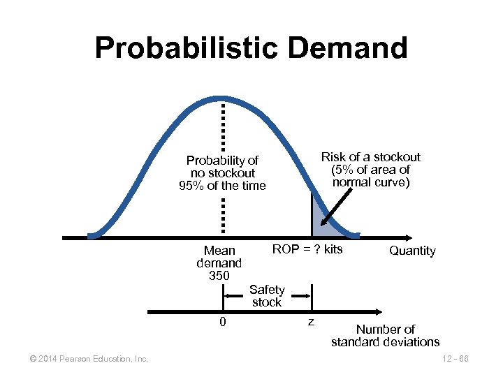 Probabilistic Demand Risk of a stockout (5% of area of normal curve) Probability of no stockout 95% of the time Mean demand 350 0 © 2014 Pearson Education, Inc. ROP = ? kits Quantity Safety stock z Number of standard deviations 12 - 66
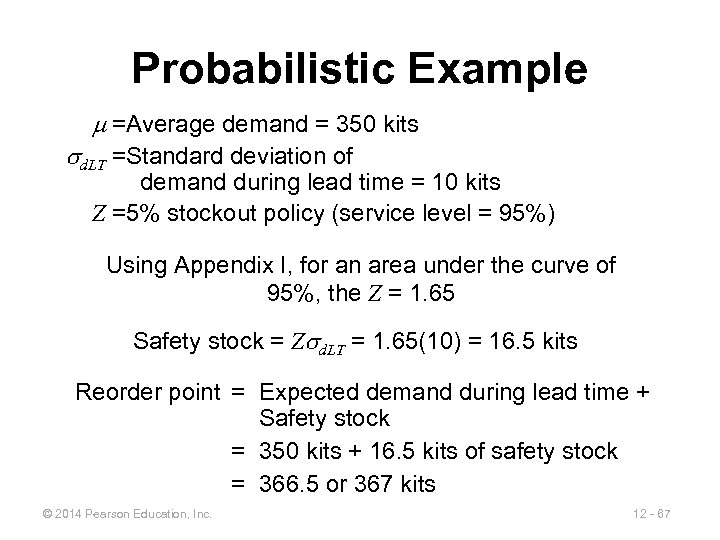 Probabilistic Example =Average demand = 350 kits d. LT =Standard deviation of demand during lead time = 10 kits Z =5% stockout policy (service level = 95%) Using Appendix I, for an area under the curve of 95%, the Z = 1. 65 Safety stock = Z d. LT = 1. 65(10) = 16. 5 kits Reorder point = Expected demand during lead time + Safety stock = 350 kits + 16. 5 kits of safety stock = 366. 5 or 367 kits © 2014 Pearson Education, Inc. 12 - 67
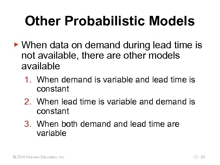 Other Probabilistic Models ▶ When data on demand during lead time is not available, there are other models available 1. When demand is variable and lead time is constant 2. When lead time is variable and demand is constant 3. When both demand lead time are variable © 2014 Pearson Education, Inc. 12 - 68
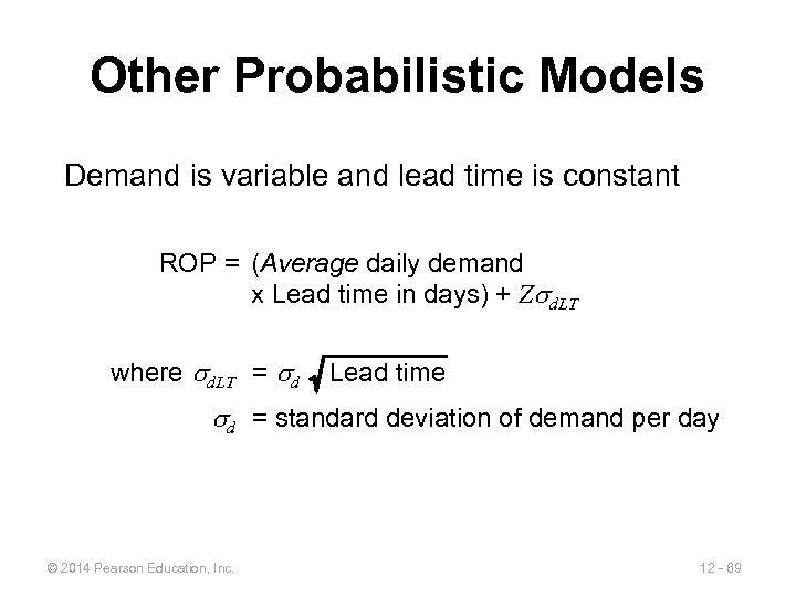 Other Probabilistic Models Demand is variable and lead time is constant ROP = (Average daily demand x Lead time in days) + Z d. LT where d. LT = d Lead time d = standard deviation of demand per day © 2014 Pearson Education, Inc. 12 - 69
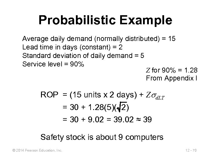 Probabilistic Example Average daily demand (normally distributed) = 15 Lead time in days (constant) = 2 Standard deviation of daily demand = 5 Service level = 90% Z for 90% = 1. 28 From Appendix I ROP = (15 units x 2 days) + Z d. LT = 30 + 1. 28(5)( 2) = 30 + 9. 02 = 39. 02 ≈ 39 Safety stock is about 9 computers © 2014 Pearson Education, Inc. 12 - 70
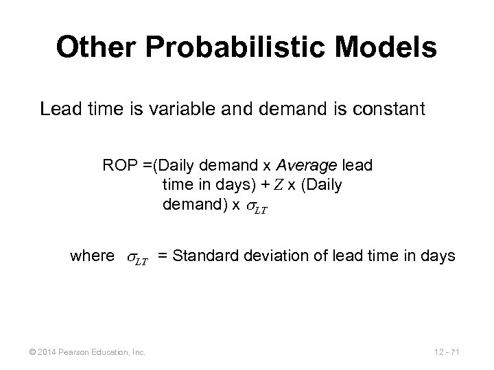 Other Probabilistic Models Lead time is variable and demand is constant ROP =(Daily demand x Average lead time in days) + Z x (Daily demand) x LT where LT = Standard deviation of lead time in days © 2014 Pearson Education, Inc. 12 - 71
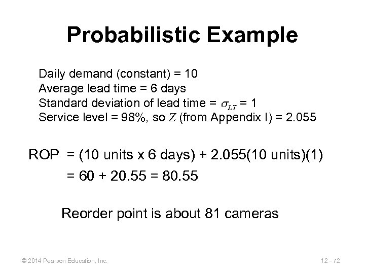 Probabilistic Example Daily demand (constant) = 10 Average lead time = 6 days Standard deviation of lead time = LT = 1 Service level = 98%, so Z (from Appendix I) = 2. 055 ROP = (10 units x 6 days) + 2. 055(10 units)(1) = 60 + 20. 55 = 80. 55 Reorder point is about 81 cameras © 2014 Pearson Education, Inc. 12 - 72
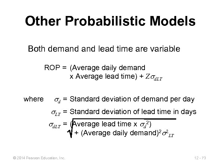 Other Probabilistic Models Both demand lead time are variable ROP = (Average daily demand x Average lead time) + Z d. LT where d = Standard deviation of demand per day LT = Standard deviation of lead time in days d. LT = (Average lead time x d 2) + (Average daily demand)2 2 LT © 2014 Pearson Education, Inc. 12 - 73
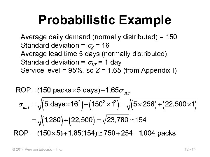 Probabilistic Example Average daily demand (normally distributed) = 150 Standard deviation = d = 16 Average lead time 5 days (normally distributed) Standard deviation = LT = 1 day Service level = 95%, so Z = 1. 65 (from Appendix I) © 2014 Pearson Education, Inc. 12 - 74
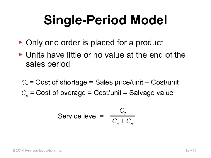 Single-Period Model ▶ Only one order is placed for a product ▶ Units have little or no value at the end of the sales period Cs = Cost of shortage = Sales price/unit – Cost/unit Co = Cost of overage = Cost/unit – Salvage value Service level = © 2014 Pearson Education, Inc. Cs Cs + Co 12 - 75
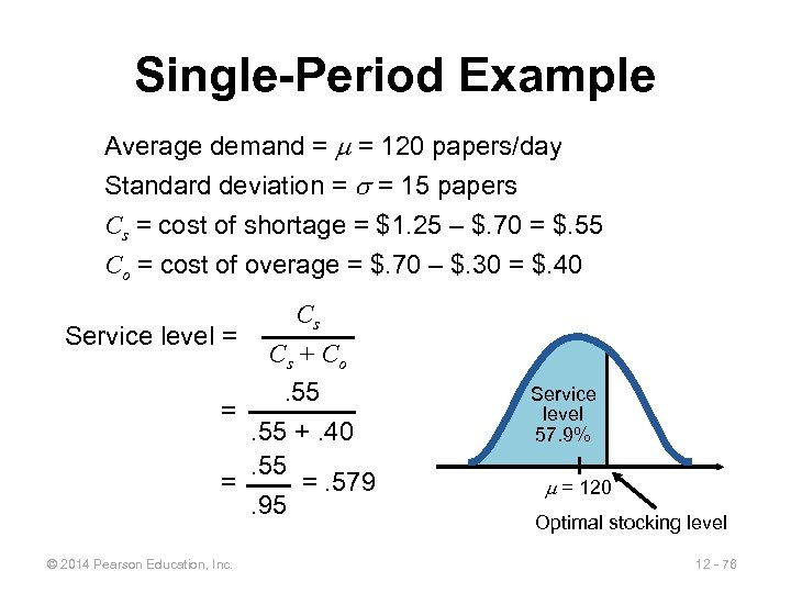 Single-Period Example Average demand = = 120 papers/day Standard deviation = = 15 papers Cs = cost of shortage = $1. 25 – $. 70 = $. 55 Co = cost of overage = $. 70 – $. 30 = $. 40 Cs Service level = Cs + Co. 55 =. 55 +. 40. 55 = =. 579. 95 © 2014 Pearson Education, Inc. Service level 57. 9% = 120 Optimal stocking level 12 - 76
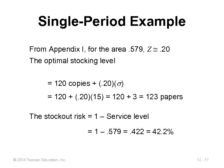 Single-Period Example From Appendix I, for the area. 579, Z . 20 The optimal stocking level = 120 copies + (. 20)( ) = 120 + (. 20)(15) = 120 + 3 = 123 papers The stockout risk = 1 – Service level = 1 –. 579 =. 422 = 42. 2% © 2014 Pearson Education, Inc. 12 - 77
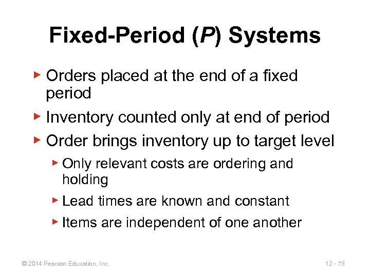 Fixed-Period (P) Systems ▶ Orders placed at the end of a fixed period ▶ Inventory counted only at end of period ▶ Order brings inventory up to target level ▶ Only relevant costs are ordering and holding ▶ Lead times are known and constant ▶ Items are independent of one another © 2014 Pearson Education, Inc. 12 - 78
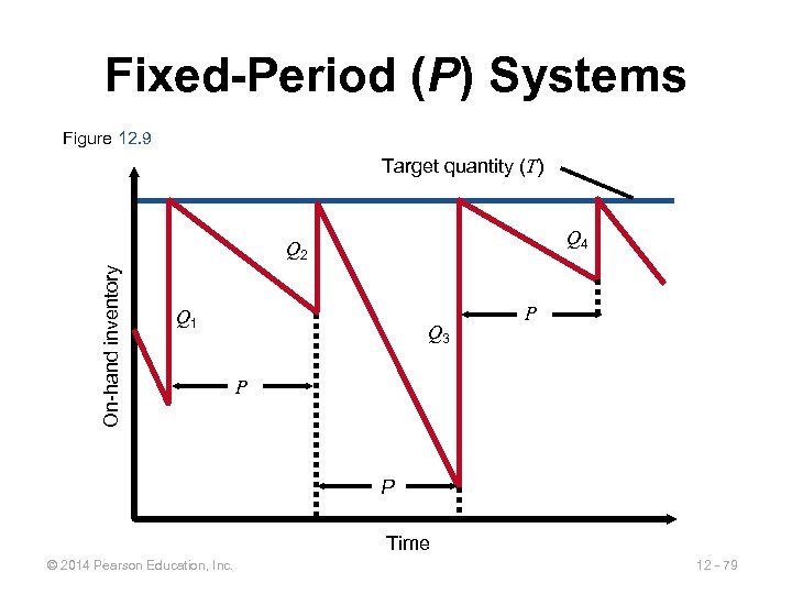 Fixed-Period (P) Systems Figure 12. 9 Target quantity (T) Q 4 On-hand inventory Q 2 Q 1 Q 3 P P P Time © 2014 Pearson Education, Inc. 12 - 79
 Fixed-Period Systems ▶ Inventory is only counted at each review period ▶ May be scheduled at convenient times ▶ Appropriate in routine situations ▶ May result in stockouts between periods ▶ May require increased safety stock © 2014 Pearson Education, Inc. 12 - 80
 All rights reserved. No part of this publication may be reproduced, stored in a retrieval system, or transmitted, in any form or by any means, electronic, mechanical, photocopying, recording, or otherwise, without the prior written permission of the publisher. Printed in the United States of America. © 2014 Pearson Education, Inc. 12 - 81
 Aggregate Planning and S&OP 13 Power. Point presentation to accompany Heizer and Render Operations Management, Eleventh Edition Principles of Operations Management, Ninth Edition Power. Point slides by Jeff Heyl © 2014 Pearson Education, Inc. © 2014 Pearson Education, 13 - 82
 Outline ► ► ► Global Company Profile: Frito-Lay The Planning Process Sales and Operations Planning The Nature of Aggregate Planning Strategies © 2014 Pearson Education, Inc. 13 - 83
 Outline - Continued ► ► ► Methods for Aggregate Planning in Services Revenue Management © 2014 Pearson Education, Inc. 13 - 84
 Learning Objectives When you complete this chapter you should be able to: 1. Define sales and operations planning 2. Define aggregate planning 3. Identify optional strategies for developing an aggregate plan © 2014 Pearson Education, Inc. 13 - 85
 Learning Objectives When you complete this chapter you should be able to: 4. Prepare a graphical aggregate plan 5. Solve an aggregate plan via the transportation method 6. Understand solve a revenue management problem © 2014 Pearson Education, Inc. 13 - 86
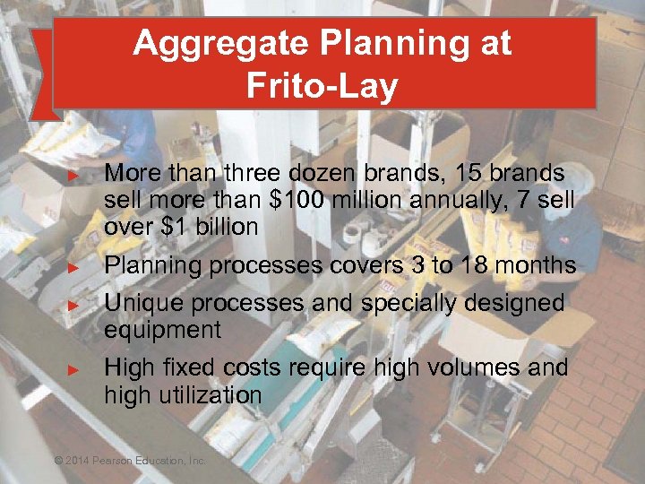 Aggregate Planning at Frito-Lay ► ► More than three dozen brands, 15 brands sell more than $100 million annually, 7 sell over $1 billion Planning processes covers 3 to 18 months Unique processes and specially designed equipment High fixed costs require high volumes and high utilization © 2014 Pearson Education, Inc. © 2014 Pearson Education, 13 - 87
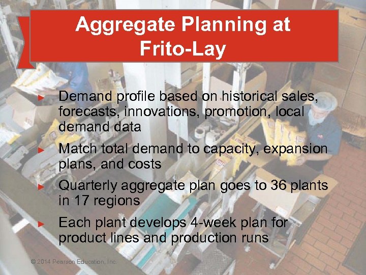 Aggregate Planning at Frito-Lay ► ► Demand profile based on historical sales, forecasts, innovations, promotion, local demand data Match total demand to capacity, expansion plans, and costs Quarterly aggregate plan goes to 36 plants in 17 regions Each plant develops 4 -week plan for product lines and production runs © 2014 Pearson Education, Inc. © 2014 Pearson Education, 13 - 88
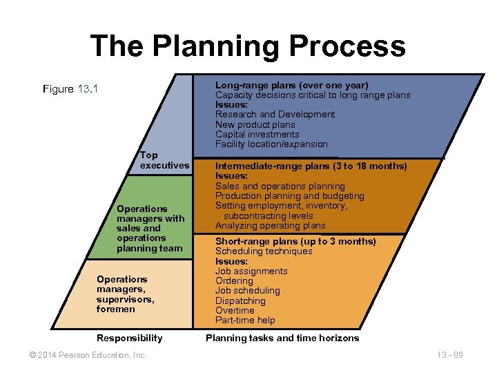 The Planning Process Long-range plans (over one year) Capacity decisions critical to long range plans Issues: Research and Development New product plans Capital investments Facility location/expansion Figure 13. 1 Top executives Operations managers with sales and operations planning team Operations managers, supervisors, foremen Responsibility © 2014 Pearson Education, Inc. Intermediate-range plans (3 to 18 months) Issues: Sales and operations planning Production planning and budgeting Setting employment, inventory, subcontracting levels Analyzing operating plans Short-range plans (up to 3 months) Scheduling techniques Issues: Job assignments Ordering Job scheduling Dispatching Overtime Part-time help Planning tasks and time horizons 13 - 89
 Sales and Operations Planning ▶ Coordination of demand forecasts with functional areas and the supply chain ▶ Typically done by cross-functional teams ▶ Determine which plans are feasible ▶ Limitations must be reflected ▶ Provides warning when resources do not match expectations ▶ Output is an aggregate plan © 2014 Pearson Education, Inc. 13 - 90
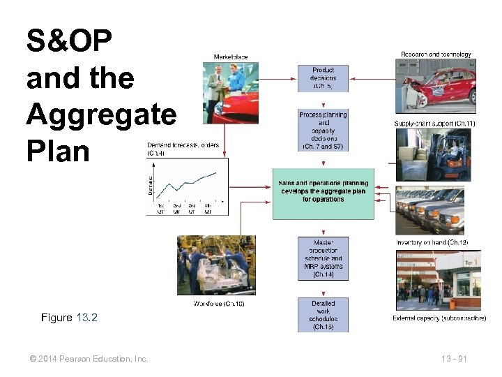 S&OP and the Aggregate Plan Figure 13. 2 © 2014 Pearson Education, Inc. 13 - 91
 Sales and Operations Planning ▶ Decisions must be tied to strategic planning and integrated with all areas of the firm over all planning horizons ▶ S&OP is aimed at 1. The coordination and integration of the internal and external resources necessary for a successful aggregate plan 2. Communication of the plan to those charged with its execution © 2014 Pearson Education, Inc. 13 - 92
 Sales and Operations Planning ▶ Requires ▶ A logical overall unit for measuring sales and output ▶ A forecast of demand for an intermediate planning period in these aggregate terms ▶ A method for determining relevant costs ▶ A model that combines forecasts and costs so that scheduling decisions can be made for the planning period © 2014 Pearson Education, Inc. 13 - 93
 Aggregate Planning The objective of aggregate planning is usually to meet forecast demand while minimizing cost over the planning period © 2014 Pearson Education, Inc. 13 - 94
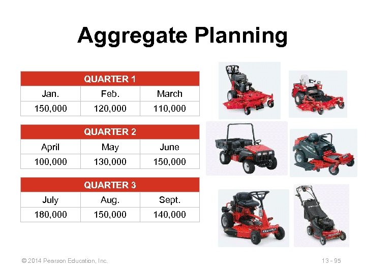 Aggregate Planning QUARTER 1 Jan. Feb. March 150, 000 120, 000 110, 000 QUARTER 2 April May June 100, 000 130, 000 150, 000 QUARTER 3 July Aug. Sept. 180, 000 150, 000 140, 000 © 2014 Pearson Education, Inc. 13 - 95
 Aggregate Planning ▶ Combines appropriate resources into general terms ▶ Part of a larger production planning system ▶ Disaggregation breaks the plan down into greater detail ▶ Disaggregation results in a master production schedule © 2014 Pearson Education, Inc. 13 - 96
 Aggregate Planning Strategies 1. Should inventories be used to absorb changes in demand? 2. Should changes be accommodated by varying the size of the workforce? 3. Should part-timers, overtime, or idle time be used to absorb changes? 4. Should subcontractors be used and maintain a stable workforce? 5. Should prices or other factors be changed to influence demand? © 2014 Pearson Education, Inc. 13 - 97
 Capacity Options 1. Changing inventory levels ▶ Increase inventory in low demand periods to meet high demand in the future ▶ Increases costs associated with storage, insurance, handling, obsolescence, and capital investment ▶ Shortages may mean lost sales due to long lead times and poor customer service © 2014 Pearson Education, Inc. 13 - 98
 Capacity Options 2. Varying workforce size by hiring or layoffs ▶ Match production rate to demand ▶ Training and separation costs for hiring and laying off workers ▶ New workers may have lower productivity ▶ Laying off workers may lower morale and productivity © 2014 Pearson Education, Inc. 13 - 99
 Capacity Options 3. Varying production rates through overtime or idle time ▶ Allows constant workforce ▶ May be difficult to meet large increases in demand ▶ Overtime can be costly and may drive down productivity ▶ Absorbing idle time may be difficult © 2014 Pearson Education, Inc. 13 - 100
 Capacity Options 4. Subcontracting ▶ Temporary measure during periods of peak demand ▶ May be costly ▶ Assuring quality and timely delivery may be difficult ▶ Exposes your customers to a possible competitor © 2014 Pearson Education, Inc. 13 - 101
 Capacity Options 5. Using part-time workers ▶ Useful for filling unskilled or low skilled positions, especially in services © 2014 Pearson Education, Inc. 13 - 102
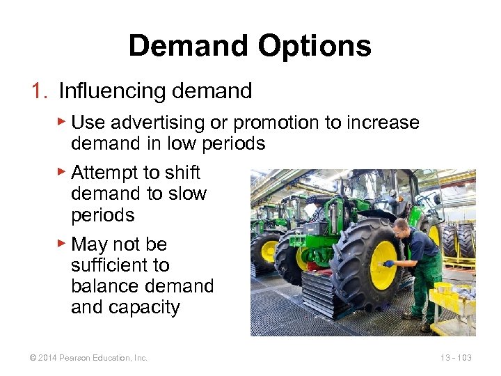 Demand Options 1. Influencing demand ▶ Use advertising or promotion to increase demand in low periods ▶ Attempt to shift demand to slow periods ▶ May not be sufficient to balance demand capacity © 2014 Pearson Education, Inc. 13 - 103
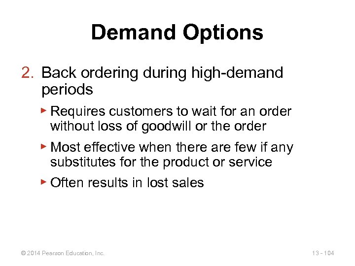 Demand Options 2. Back ordering during high-demand periods ▶ Requires customers to wait for an order without loss of goodwill or the order ▶ Most effective when there are few if any substitutes for the product or service ▶ Often results in lost sales © 2014 Pearson Education, Inc. 13 - 104
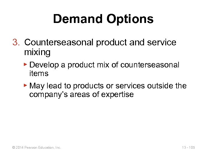 Demand Options 3. Counterseasonal product and service mixing ▶ Develop a product mix of counterseasonal items ▶ May lead to products or services outside the company’s areas of expertise © 2014 Pearson Education, Inc. 13 - 105
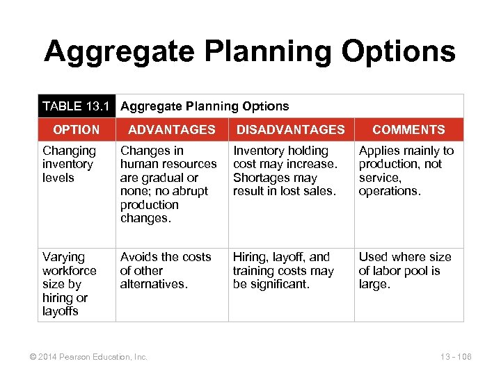 Aggregate Planning Options TABLE 13. 1 Aggregate Planning Options OPTION ADVANTAGES DISADVANTAGES COMMENTS Changing inventory levels Changes in human resources are gradual or none; no abrupt production changes. Inventory holding cost may increase. Shortages may result in lost sales. Applies mainly to production, not service, operations. Varying workforce size by hiring or layoffs Avoids the costs of other alternatives. Hiring, layoff, and training costs may be significant. Used where size of labor pool is large. © 2014 Pearson Education, Inc. 13 - 106
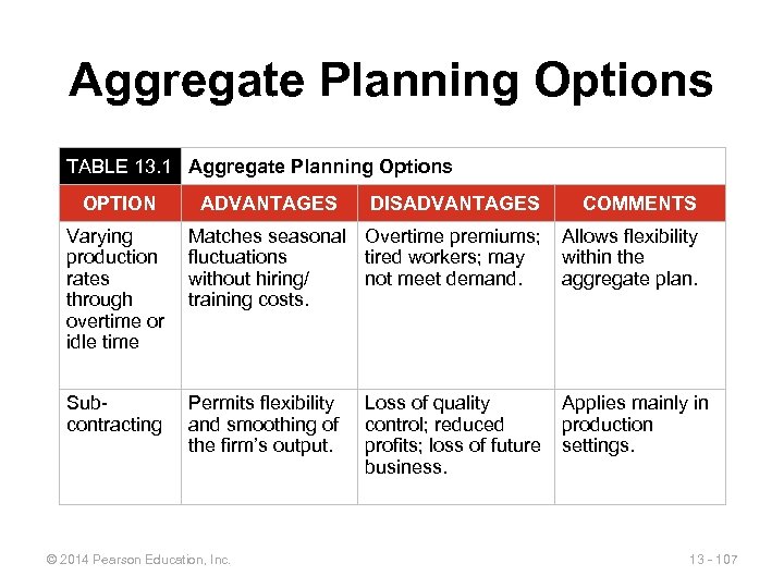 Aggregate Planning Options TABLE 13. 1 Aggregate Planning Options OPTION ADVANTAGES DISADVANTAGES COMMENTS Varying production rates through overtime or idle time Matches seasonal Overtime premiums; fluctuations tired workers; may without hiring/ not meet demand. training costs. Allows flexibility within the aggregate plan. Subcontracting Permits flexibility and smoothing of the firm’s output. Applies mainly in production settings. © 2014 Pearson Education, Inc. Loss of quality control; reduced profits; loss of future business. 13 - 107
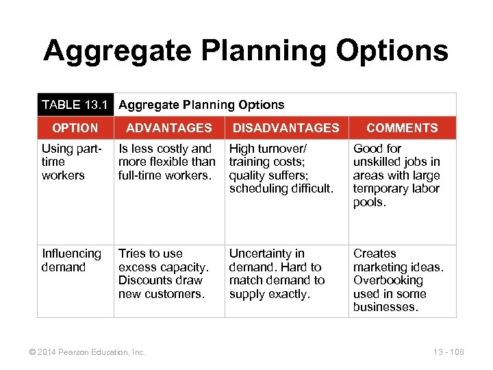 Aggregate Planning Options TABLE 13. 1 Aggregate Planning Options OPTION ADVANTAGES Using parttime workers Is less costly and more flexible than full-time workers. High turnover/ training costs; quality suffers; scheduling difficult. Good for unskilled jobs in areas with large temporary labor pools. Influencing demand Tries to use excess capacity. Discounts draw new customers. Uncertainty in demand. Hard to match demand to supply exactly. Creates marketing ideas. Overbooking used in some businesses. © 2014 Pearson Education, Inc. DISADVANTAGES COMMENTS 13 - 108
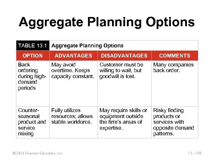 Aggregate Planning Options TABLE 13. 1 Aggregate Planning Options OPTION ADVANTAGES DISADVANTAGES COMMENTS Back May avoid ordering overtime. Keeps during high- capacity constant. demand periods Customer must be willing to wait, but goodwill is lost. Many companies back order. Counter. Fully utilizes seasonal resources; allows product and stable workforce. service mixing May require skills or equipment outside the firm’s areas of expertise. Risky finding products or services with opposite demand patterns. © 2014 Pearson Education, Inc. 13 - 109
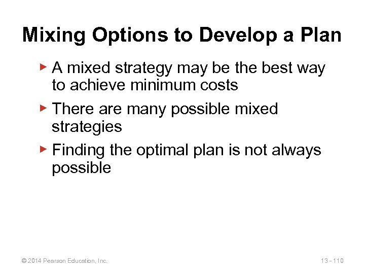 Mixing Options to Develop a Plan ▶ A mixed strategy may be the best way to achieve minimum costs ▶ There are many possible mixed strategies ▶ Finding the optimal plan is not always possible © 2014 Pearson Education, Inc. 13 - 110
 Mixing Options to Develop a Plan ▶ Chase strategy ▶ Match output rates to demand forecast for each period ▶ Vary workforce levels or vary production rate ▶ Favored by many service organizations © 2014 Pearson Education, Inc. 13 - 111
 Mixing Options to Develop a Plan ▶ Level strategy ▶ Daily production is uniform ▶ Use inventory or idle time as buffer ▶ Stable production leads to better quality and productivity ▶ Some combination of capacity options, a mixed strategy, might be the best solution © 2014 Pearson Education, Inc. 13 - 112
 Methods for Aggregate Planning ▶ Graphical Methods ▶ Popular techniques ▶ Easy to understand use ▶ Trial-and-error approaches that do not guarantee an optimal solution ▶ Require only limited computations © 2014 Pearson Education, Inc. 13 - 113
 Graphical Methods 1. Determine the demand for each period 2. Determine the capacity for regular time, overtime, and subcontracting each period 3. Find labor costs, hiring and layoff costs, and inventory holding costs 4. Consider company policy on workers and stock levels 5. Develop alternative plans and examine their total cost © 2014 Pearson Education, Inc. 13 - 114
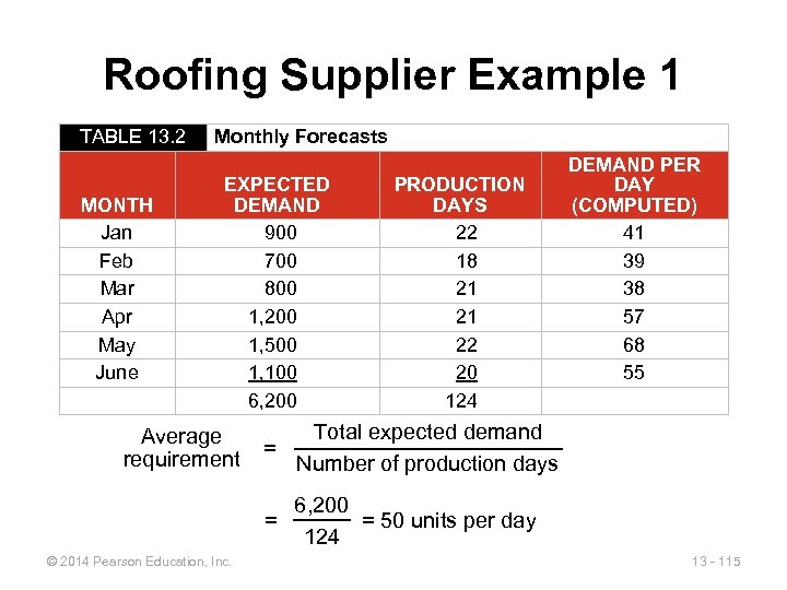 Roofing Supplier Example 1 TABLE 13. 2 MONTH Jan Feb Mar Apr May June Monthly Forecasts EXPECTED DEMAND 900 700 800 1, 200 1, 500 1, 100 6, 200 Average requirement Total expected demand = Number of production days = © 2014 Pearson Education, Inc. PRODUCTION DAYS 22 18 21 21 22 20 124 DEMAND PER DAY (COMPUTED) 41 39 38 57 68 55 6, 200 = 50 units per day 124 13 - 115
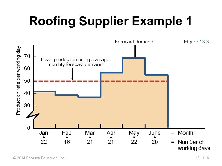 Roofing Supplier Example 1 Figure 13. 3 Production rate per working day Forecast demand 70 – 60 – Level production using average monthly forecast demand 50 – 40 – 30 – Jan Feb Mar Apr May June 22 18 21 21 22 20 © 2014 Pearson Education, Inc. = Month = Number of working days 13 - 116
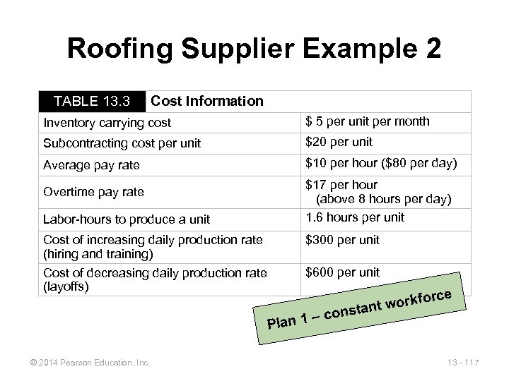 Roofing Supplier Example 2 TABLE 13. 3 Cost Information Inventory carrying cost $ 5 per unit per month Subcontracting cost per unit $20 per unit Average pay rate $10 per hour ($80 per day) Overtime pay rate Labor-hours to produce a unit Cost of increasing daily production rate (hiring and training) Cost of decreasing daily production rate (layoffs) $17 per hour (above 8 hours per day) 1. 6 hours per unit $300 per unit $600 per unit – Plan 1 © 2014 Pearson Education, Inc. rce con kfo nt wor sta 13 - 117
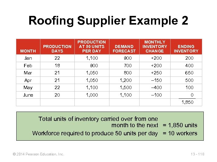 Roofing Supplier Example 2 MONTH PRODUCTION DAYS PRODUCTION AT 50 UNITS PER DAY Jan 22 1, 100 900 +200 Feb 18 900 700 +200 400 Mar 21 1, 050 800 +250 650 Apr 21 1, 050 1, 200 – 150 500 May 22 1, 100 1, 500 – 400 100 June 20 1, 000 1, 100 – 100 0 DEMAND FORECAST MONTHLY INVENTORY CHANGE ENDING INVENTORY 1, 850 Total units of inventory carried over from one month to the next = 1, 850 units Workforce required to produce 50 units per day = 10 workers © 2014 Pearson Education, Inc. 13 - 118
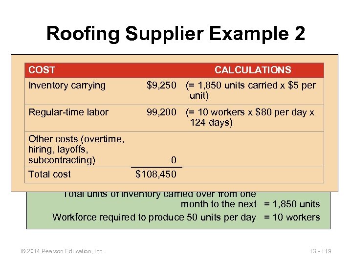 Roofing Supplier Example 2 COST PRODUCTION MONTH DAYS Inventory carrying Jan 22 Feb 18 Mar 21 Apr 21 Regular-time labor Other costs (overtime, May 22 hiring, layoffs, 20 June subcontracting) Total cost PRODUCTION MONTHLY CALCULATIONS DEMAND ENDING AT 50 UNITS INVENTORY PER$9, 250 FORECAST units carried x $5 per DAY INVENTORY (= 1, 850 CHANGE 1, 100 900 unit) +200 900 700 +200 400 1, 050 1, 200 – 150 500 1, 100 1, 500 – 400 1, 000 1, 100 – 100 0 99, 200 (= 10 workers x $80 per day x 1, 050 800 650 124 days) +250 0 $108, 450 1, 850 Total units of inventory carried over from one month to the next = 1, 850 units Workforce required to produce 50 units per day = 10 workers © 2014 Pearson Education, Inc. 13 - 119
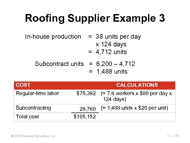 Roofing Supplier Example 3 In-house production = 38 units per day x 124 days = 4, 712 units Subcontract units = 6, 200 – 4, 712 = 1, 488 units COST Regular-time labor Subcontracting Total cost © 2014 Pearson Education, Inc. CALCULATIONS $75, 392 (= 7. 6 workers x $80 per day x 124 days) 29, 760 (= 1, 488 units x $20 per unit) $105, 152 13 - 120
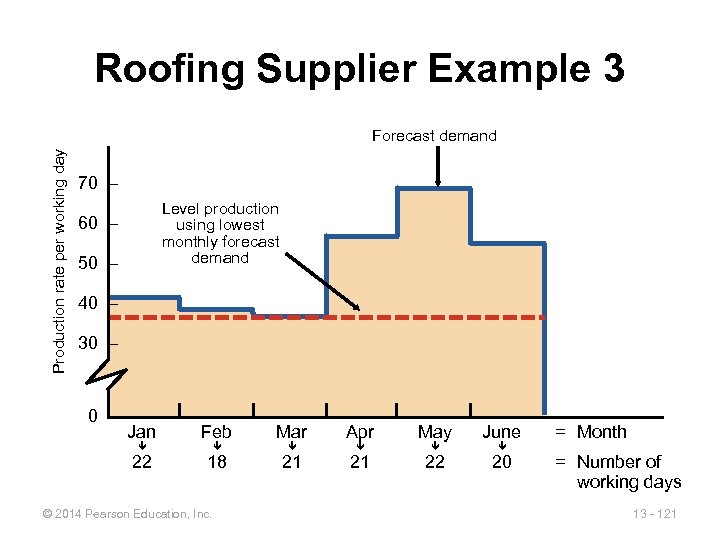 Roofing Supplier Example 3 Production rate per working day Forecast demand 70 – Level production using lowest monthly forecast demand 60 – 50 – 40 – 30 – Jan Feb Mar Apr May June 22 18 21 21 22 20 © 2014 Pearson Education, Inc. = Month = Number of working days 13 - 121
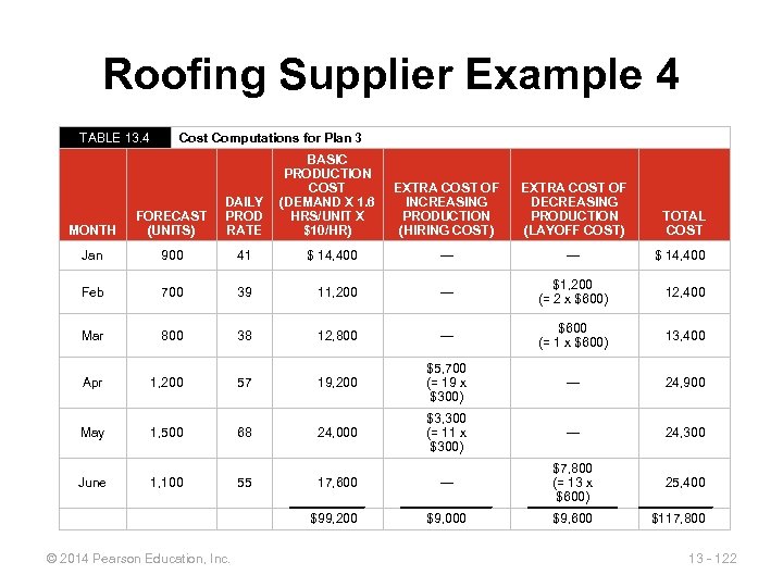 Roofing Supplier Example 4 TABLE 13. 4 Cost Computations for Plan 3 BASIC PRODUCTION COST (DEMAND X 1. 6 HRS/UNIT X $10/HR) EXTRA COST OF INCREASING PRODUCTION (HIRING COST) EXTRA COST OF DECREASING PRODUCTION (LAYOFF COST) MONTH FORECAST (UNITS) DAILY PROD RATE Jan 900 41 $ 14, 400 — — Feb 700 39 11, 200 — $1, 200 (= 2 x $600) 12, 400 Mar 800 38 12, 800 — $600 (= 1 x $600) 13, 400 Apr 1, 200 57 19, 200 $5, 700 (= 19 x $300) — 24, 900 May 1, 500 68 24, 000 $3, 300 (= 11 x $300) — 24, 300 17, 600 — $7, 800 (= 13 x $600) 25, 400 $99, 200 $9, 000 $9, 600 $117, 800 June 1, 100 © 2014 Pearson Education, Inc. 55 TOTAL COST $ 14, 400 13 - 122
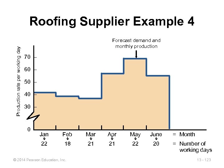 Production rate per working day Roofing Supplier Example 4 Forecast demand monthly production 70 – 60 – 50 – 40 – 30 – Jan Feb Mar Apr May June 22 18 21 21 22 20 © 2014 Pearson Education, Inc. = Month = Number of working days 13 - 123
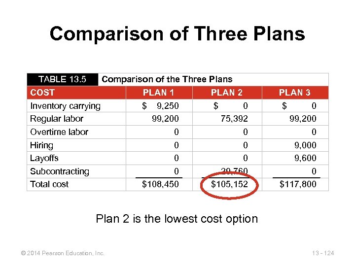 Comparison of Three Plans TABLE 13. 5 Comparison of the Three Plans COST PLAN 1 PLAN 2 Inventory carrying $ 9, 250 $ 0 Regular labor 99, 200 75, 392 Overtime labor 0 0 Hiring 0 0 Layoffs 0 0 Subcontracting 0 29, 760 Total cost $108, 450 $105, 152 PLAN 3 $ 0 99, 200 0 9, 000 9, 600 0 $117, 800 Plan 2 is the lowest cost option © 2014 Pearson Education, Inc. 13 - 124
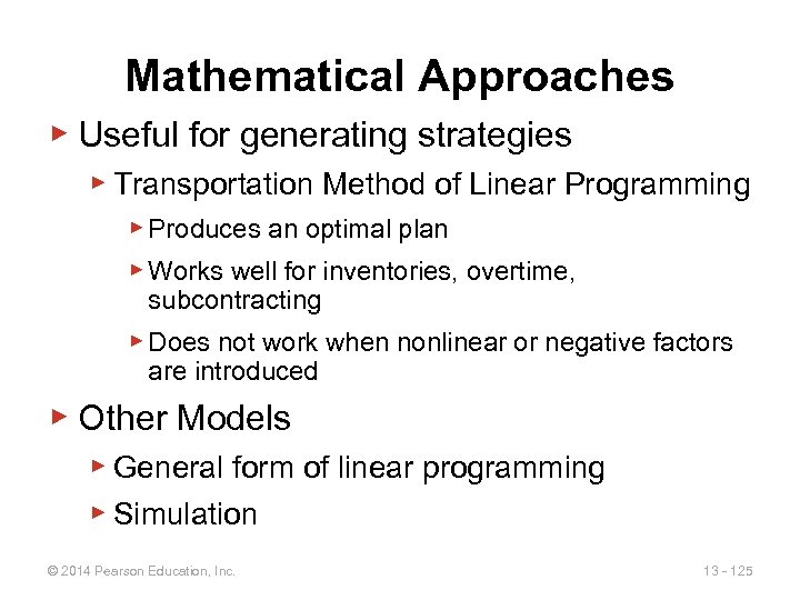 Mathematical Approaches ▶ Useful for generating strategies ▶ Transportation Method of Linear Programming ▶ Produces an optimal plan ▶ Works well for inventories, overtime, subcontracting ▶ Does not work when nonlinear or negative factors are introduced ▶ Other Models ▶ General form of linear programming ▶ Simulation © 2014 Pearson Education, Inc. 13 - 125
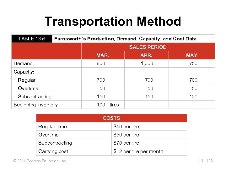 Transportation Method TABLE 13. 6 Farnsworth’s Production, Demand, Capacity, and Cost Data SALES PERIOD MAR. APR. MAY 800 1, 000 750 Regular 700 700 Overtime 50 50 50 150 130 Demand Capacity: Subcontracting Beginning inventory 100 tires COSTS Regular time $40 per tire Overtime $50 per tire Subcontracting $70 per tire Carrying cost $ 2 per tire per month © 2014 Pearson Education, Inc. 13 - 126
 Transportation Example ▶ Important points 1. Carrying costs are $2/tire/month. If goods are made in one period and held over to the next, holding costs are incurred. 2. Supply must equal demand, so a dummy column called “unused capacity” is added. 3. Because back ordering is not viable in this example, cells that might be used to satisfy earlier demand are not available. © 2014 Pearson Education, Inc. 13 - 127
 Transportation Example 4. Quantities in each column designate the levels of inventory needed to meet demand requirements 5. In general, production should be allocated to the lowest cost cell available without exceeding unused capacity in the row or demand in the column © 2014 Pearson Education, Inc. 13 - 128
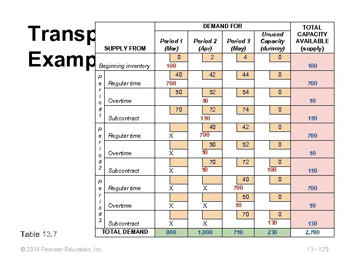 Transportation Example SUPPLY FROM Beginning inventory P e r i o d 1 Regular time Overtime Table 13. 7 Period 2 (Apr) 2 Period 3 (May) 4 42 44 700 52 54 Overtime 72 74 X 150 40 700 X 0 150 42 52 0 700 0 50 50 70 Subcontract 0 50 50 X 72 50 0 100 150 Overtime X X 40 700 0 50 Regular time 0 700 50 50 70 Subcontract TOTAL DEMAND © 2014 Pearson Education, Inc. TOTAL CAPACITY AVAILABLE (supply) 0 50 Subcontract Regular time Unused Capacity (dummy) 0 100 70 P e r i o d 2 P e r i o d 3 Period 1 (Mar) 0 100 40 700 50 DEMAND FOR X 1, 000 130 X 800 0 750 130 2, 780 13 - 129
 Aggregate Planning in Services ▶ Most services use combination strategies and mixed plans ▶ Controlling the cost of labor is critical 1. Accurate scheduling of labor-hours to assure quick response to customer demand 2. An on-call labor resource to cover unexpected demand 3. Flexibility of individual worker skills 4. Flexibility in rate of output or hours of work © 2014 Pearson Education, Inc. 13 - 130
 Five Service Scenarios ▶ Restaurants 1. Smoothing the production process 2. Determining the optimal workforce size ▶ Hospitals ▶ Responding to patient demand ▶ National Chains of Small Service Firms ▶ Planning done at national level and at local level © 2014 Pearson Education, Inc. 13 - 131
 Five Service Scenarios ▶ Miscellaneous Services ▶ Plan human resource requirements ▶ Manage demand ▶ Airline industry ▶ Extremely complex planning problem ▶ Involves number of flights, number of passengers, air and ground personnel, allocation of seats to fare classes ▶ Resources spread through the entire system © 2014 Pearson Education, Inc. 13 - 132
 Revenue Management ▶ Allocating resources to customers at prices that will maximize revenue 1. Service or product can be sold in advance of consumption 2. Demand fluctuates 3. Capacity is relatively fixed 4. Demand can be segmented 5. Variable costs are low and fixed costs are high © 2014 Pearson Education, Inc. 13 - 133
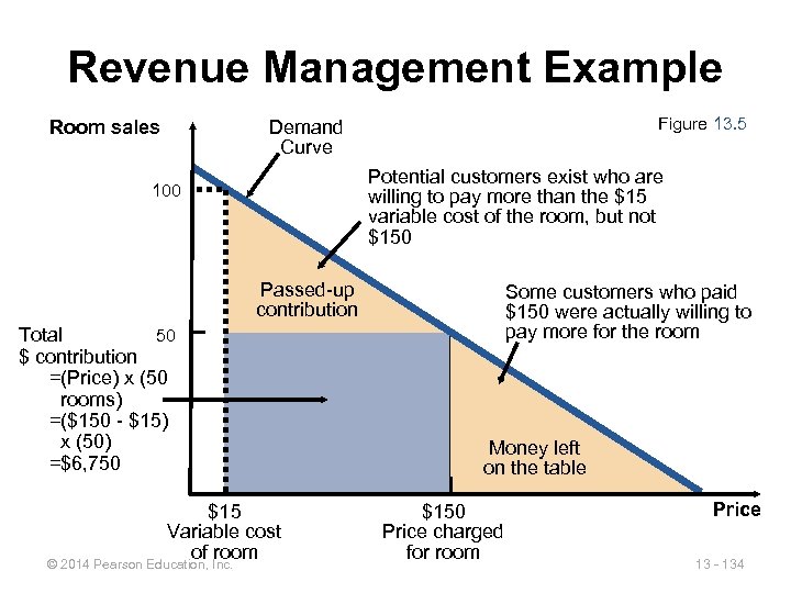 Revenue Management Example Figure 13. 5 Demand Curve Room sales Potential customers exist who are willing to pay more than the $15 variable cost of the room, but not $150 100 Passed-up contribution 50 Total $ contribution =(Price) x (50 rooms) =($150 - $15) x (50) =$6, 750 $15 Variable cost of room © 2014 Pearson Education, Inc. Some customers who paid $150 were actually willing to pay more for the room Money left on the table $150 Price charged for room Price 13 - 134
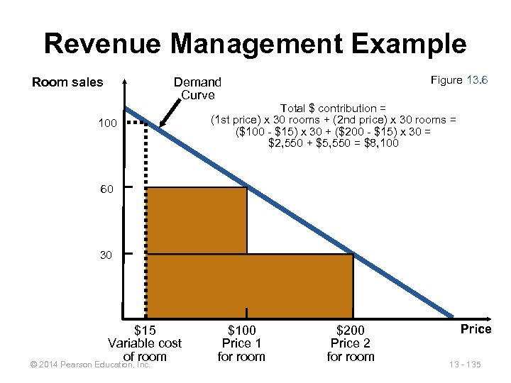 Revenue Management Example Figure 13. 6 Demand Curve Room sales 100 Total $ contribution = (1 st price) x 30 rooms + (2 nd price) x 30 rooms = ($100 - $15) x 30 + ($200 - $15) x 30 = $2, 550 + $5, 550 = $8, 100 60 30 $15 Variable cost of room © 2014 Pearson Education, Inc. $100 Price 1 for room $200 Price 2 for room Price 13 - 135
 Revenue Management Approaches ▶ Airlines, hotels, rental cars, etc. ▶ Tend to have predictable duration of service and use variable pricing to control availability and revenue ▶ Movies, stadiums, performing arts centers ▶ Tend to have predicable duration and fixed prices but use seating locations and times to manage revenue © 2014 Pearson Education, Inc. 13 - 136
 Revenue Management Approaches ▶ Restaurants, golf courses, ISPs ▶ Generally have unpredictable duration of customer use and fixed prices, may use “offpeak” rates to shift demand manage revenue ▶ Health care businesses, etc. ▶ Tend to have unpredictable duration of service and variable pricing, often attempt to control duration of service © 2014 Pearson Education, Inc. 13 - 137
 Making Revenue Management Work 1. Multiple pricing structures must be feasible and appear logical to the customer 2. Forecasts of the use and duration of use 3. Changes in demand © 2014 Pearson Education, Inc. 13 - 138
 All rights reserved. No part of this publication may be reproduced, stored in a retrieval system, or transmitted, in any form or by any means, electronic, mechanical, photocopying, recording, or otherwise, without the prior written permission of the publisher. Printed in the United States of America. © 2014 Pearson Education, Inc. 13 - 139


