UNIT 3 Classification Basic Concepts n Supervised learning

UNIT 3. Classification: Basic Concepts n Supervised learning (classification) n Supervision: The training data (observations, measurements, etc. ) are accompanied by labels indicating the class of the observations n n New data is classified based on the training set Unsupervised learning (clustering) n The class labels of training data is unknown n Given a set of measurements, observations, etc. with the aim of establishing the existence of classes or clusters in the data 1

Classification vs. Numeric Prediction n Classification n predicts categorical class labels (discrete or nominal) n classifies data (constructs a model) based on the training set and the values (class labels) in a classifying attribute and uses it in classifying new data Numeric Prediction n models continuous-valued functions, i. e. , predicts unknown or missing values Typical applications n Credit/loan approval: n Medical diagnosis: if a tumor is cancerous or benign n Fraud detection: if a transaction is fraudulent n Web page categorization: which category it is 2

Classification—A Two-Step Process n n n Model construction: describing a set of predetermined classes n Each tuple/sample is assumed to belong to a predefined class, as determined by the class label attribute n The set of tuples used for model construction is training set n The model is represented as classification rules, decision trees, or mathematical formulae Model usage: for classifying future or unknown objects n Estimate accuracy of the model n The known label of test sample is compared with the classified result from the model n Accuracy rate is the percentage of test set samples that are correctly classified by the model n Test set is independent of training set (otherwise overfitting) n If the accuracy is acceptable, use the model to classify new data Note: If the test set is used to select models, it is called validation (test) set 3

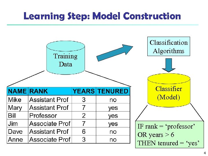
Learning Step: Model Construction Training Data Classification Algorithms Classifier (Model) IF rank = ‘professor’ OR years > 6 THEN tenured = ‘yes’ 4

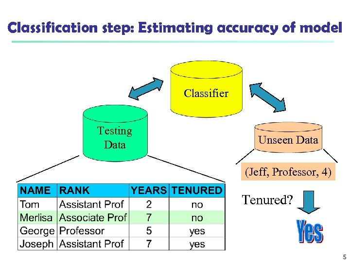
Classification step: Estimating accuracy of model Classifier Testing Data Unseen Data (Jeff, Professor, 4) Tenured? 5

Algorithm for Decision Tree Induction n n Basic algorithm (a greedy algorithm) n Tree is constructed in a top-down recursive divide-and-conquer manner n At start, all the training examples are at the root n Attributes are categorical (if continuous-valued, they are discretized in advance) n Examples are partitioned recursively based on selected attributes n Test attributes are selected on the basis of a heuristic or statistical measure (e. g. , information gain) Conditions for stopping partitioning n All samples for a given node belong to the same class n There are no remaining attributes for further partitioning – majority voting is employed for classifying the leaf n There are no samples left 6

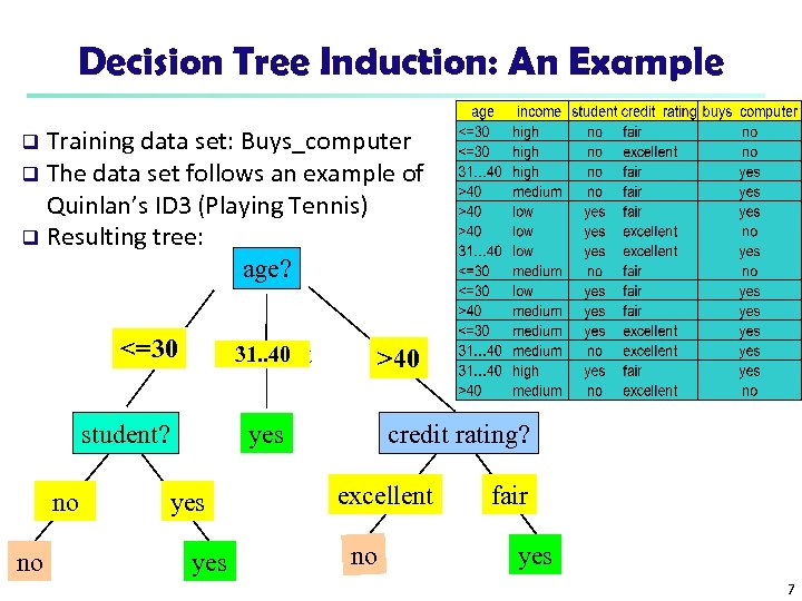
Decision Tree Induction: An Example Training data set: Buys_computer q The data set follows an example of Quinlan’s ID 3 (Playing Tennis) q Resulting tree: age? q <=30 31. . 40 overcast student? no no >40 credit rating? yes yes excellent no fair yes 7

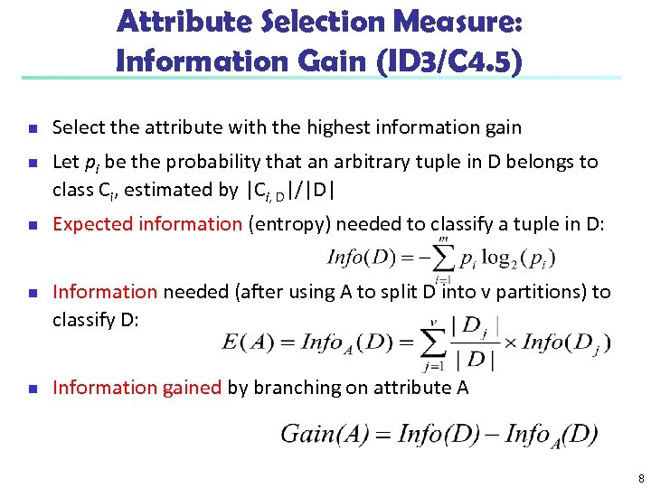
Attribute Selection Measure: Information Gain (ID 3/C 4. 5) n n n Select the attribute with the highest information gain Let pi be the probability that an arbitrary tuple in D belongs to class Ci, estimated by |Ci, D|/|D| Expected information (entropy) needed to classify a tuple in D: Information needed (after using A to split D into v partitions) to classify D: Information gained by branching on attribute A 8

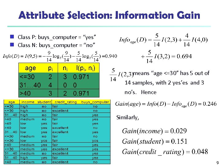
Attribute Selection: Information Gain Class P: buys_computer = “yes” g Class N: buys_computer = “no” g means “age <=30” has 5 out of 14 samples, with 2 yes’es and 3 no’s. Hence Similarly, 9

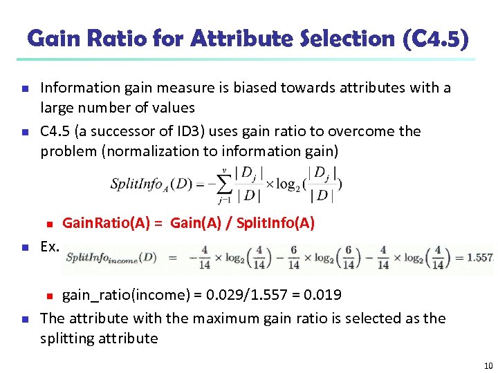
Gain Ratio for Attribute Selection (C 4. 5) n n Information gain measure is biased towards attributes with a large number of values C 4. 5 (a successor of ID 3) uses gain ratio to overcome the problem (normalization to information gain) n Gain. Ratio(A) = Gain(A) / Split. Info(A) n Ex. n gain_ratio(income) = 0. 029/1. 557 = 0. 019 The attribute with the maximum gain ratio is selected as the splitting attribute n 10

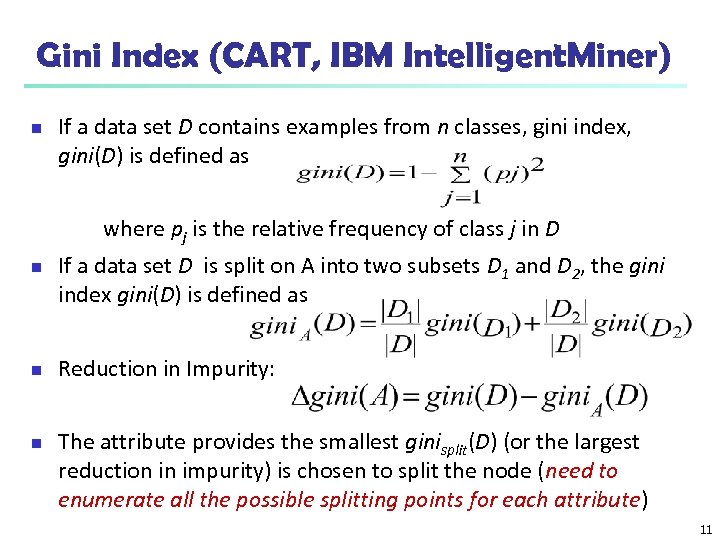
Gini Index (CART, IBM Intelligent. Miner) n If a data set D contains examples from n classes, gini index, gini(D) is defined as where pj is the relative frequency of class j in D n n n If a data set D is split on A into two subsets D 1 and D 2, the gini index gini(D) is defined as Reduction in Impurity: The attribute provides the smallest ginisplit(D) (or the largest reduction in impurity) is chosen to split the node (need to enumerate all the possible splitting points for each attribute) 11

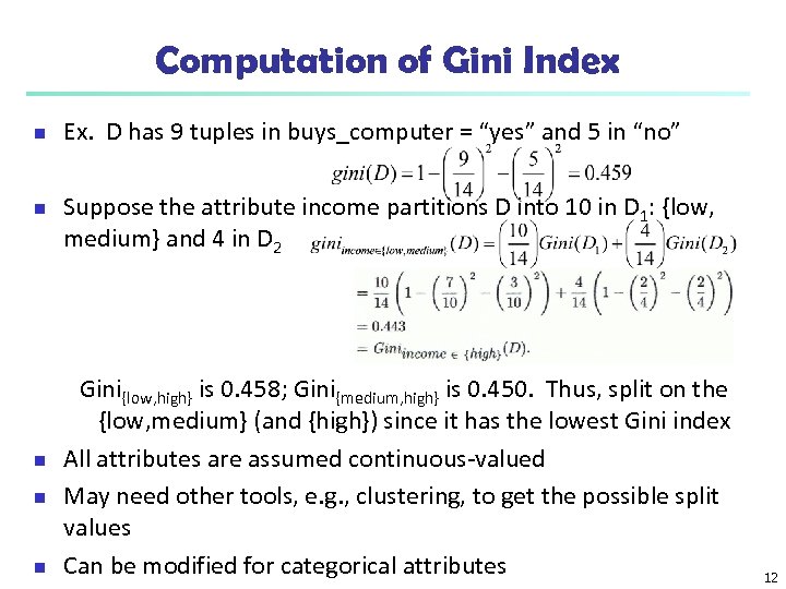
Computation of Gini Index n n n Ex. D has 9 tuples in buys_computer = “yes” and 5 in “no” Suppose the attribute income partitions D into 10 in D 1: {low, medium} and 4 in D 2 Gini{low, high} is 0. 458; Gini{medium, high} is 0. 450. Thus, split on the {low, medium} (and {high}) since it has the lowest Gini index All attributes are assumed continuous-valued May need other tools, e. g. , clustering, to get the possible split values Can be modified for categorical attributes 12

Overfitting and Tree Pruning n n Overfitting: An induced tree may overfit the training data n Too many branches, some may reflect anomalies due to noise or outliers n Poor accuracy for unseen samples Two approaches to avoid overfitting n Prepruning: Halt tree construction early do not split a node if this would result in the goodness measure falling below a threshold n Difficult to choose an appropriate threshold n Postpruning: Remove branches from a “fully grown” tree— get a sequence of progressively pruned trees n Use a set of data different from the training data to decide which is the “best pruned tree” 13

Bayesian Classification: Why? n n A statistical classifier: performs probabilistic prediction, i. e. , predicts class membership probabilities. (the probability that given tuple belongs to a particular class) Foundation: Based on Bayes’ Theorem. There are two types of Bayesian classification methods. (i) Naïve Bayesian classifier : A simple Bayesian classifier, has comparable performance with decision tree and selected neural network classifiers. This classifier assume that the effect of an attribute value on a given class is independent of the values of other attributes. (class conditional independence) (ii) Bayesian belief networks: These are graphical models, which allows the representation of dependencies among subsets of attributes. 14

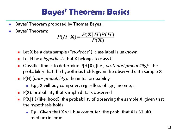
Bayes’ Theorem: Basics n n Bayes’ Theorem proposed by Thomas Bayes’ Theorem: n n n Let X be a data sample (“evidence”): class label is unknown Let H be a hypothesis that X belongs to class C Classification is to determine P(H|X), (i. e. , posteriori probability): the probability that the hypothesis holds given the observed data sample X P(H) (prior probability): the initial probability n E. g. , X will buy computer, regardless of age, income, … P(X): probability that sample data is observed P(X|H) (likelihood): the probability of observing the sample X, given that the hypothesis holds n E. g. , Given that X will buy computer, the prob. that X is 31. . 40, medium income 15

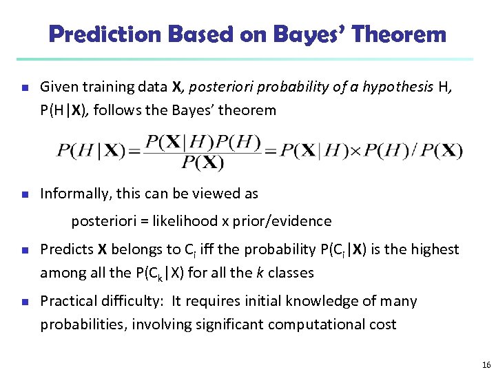
Prediction Based on Bayes’ Theorem n n Given training data X, posteriori probability of a hypothesis H, P(H|X), follows the Bayes’ theorem Informally, this can be viewed as posteriori = likelihood x prior/evidence n n Predicts X belongs to Ci iff the probability P(Ci|X) is the highest among all the P(Ck|X) for all the k classes Practical difficulty: It requires initial knowledge of many probabilities, involving significant computational cost 16

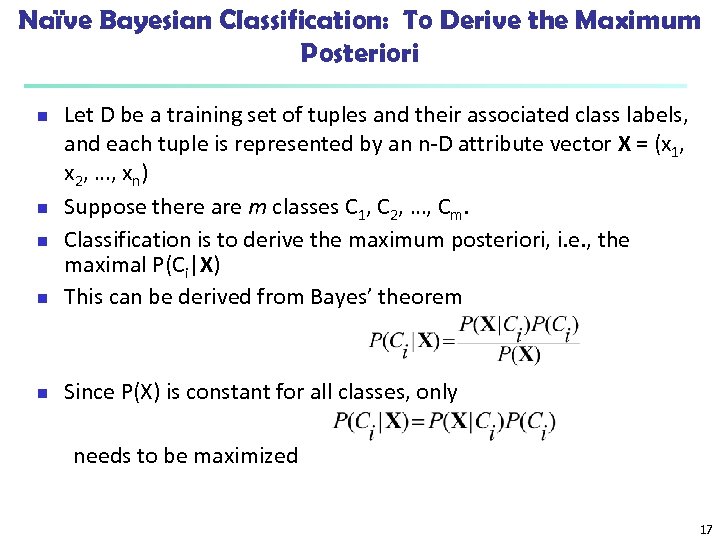
Naïve Bayesian Classification: To Derive the Maximum Posteriori n Let D be a training set of tuples and their associated class labels, and each tuple is represented by an n-D attribute vector X = (x 1, x 2, …, xn) Suppose there are m classes C 1, C 2, …, Cm. Classification is to derive the maximum posteriori, i. e. , the maximal P(Ci|X) This can be derived from Bayes’ theorem n Since P(X) is constant for all classes, only n needs to be maximized 17

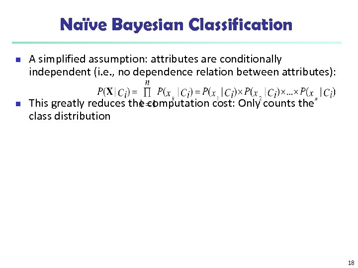
Naïve Bayesian Classification n n A simplified assumption: attributes are conditionally independent (i. e. , no dependence relation between attributes): This greatly reduces the computation cost: Only counts the class distribution 18

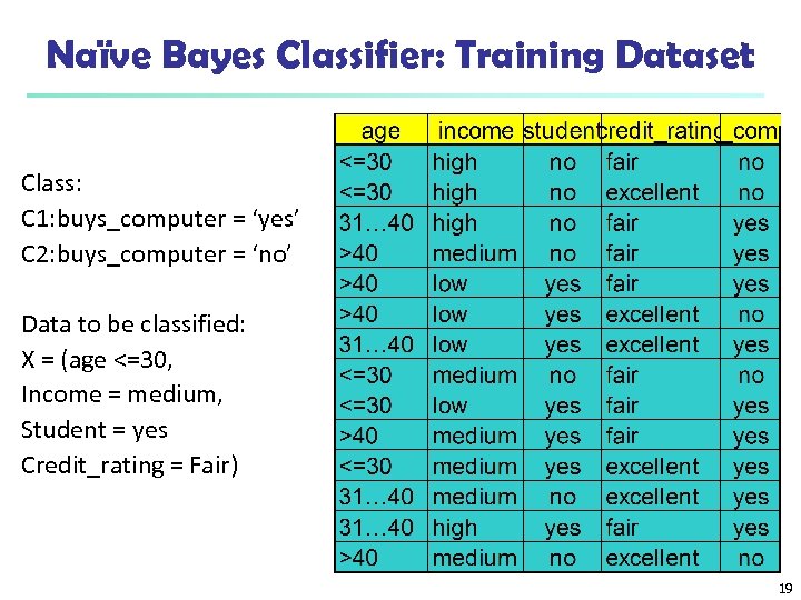
Naïve Bayes Classifier: Training Dataset Class: C 1: buys_computer = ‘yes’ C 2: buys_computer = ‘no’ Data to be classified: X = (age <=30, Income = medium, Student = yes Credit_rating = Fair) 19

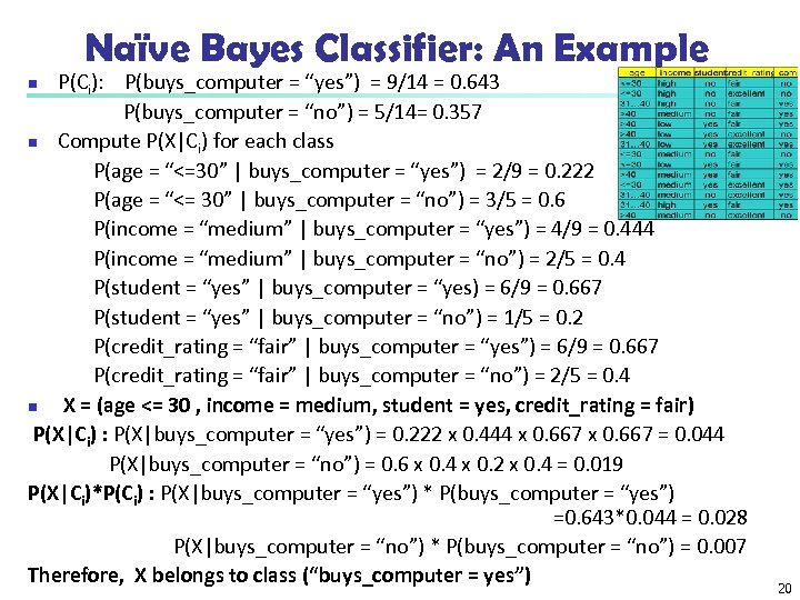
Naïve Bayes Classifier: An Example P(Ci): P(buys_computer = “yes”) = 9/14 = 0. 643 P(buys_computer = “no”) = 5/14= 0. 357 n Compute P(X|Ci) for each class P(age = “<=30” | buys_computer = “yes”) = 2/9 = 0. 222 P(age = “<= 30” | buys_computer = “no”) = 3/5 = 0. 6 P(income = “medium” | buys_computer = “yes”) = 4/9 = 0. 444 P(income = “medium” | buys_computer = “no”) = 2/5 = 0. 4 P(student = “yes” | buys_computer = “yes) = 6/9 = 0. 667 P(student = “yes” | buys_computer = “no”) = 1/5 = 0. 2 P(credit_rating = “fair” | buys_computer = “yes”) = 6/9 = 0. 667 P(credit_rating = “fair” | buys_computer = “no”) = 2/5 = 0. 4 n X = (age <= 30 , income = medium, student = yes, credit_rating = fair) P(X|Ci) : P(X|buys_computer = “yes”) = 0. 222 x 0. 444 x 0. 667 = 0. 044 P(X|buys_computer = “no”) = 0. 6 x 0. 4 x 0. 2 x 0. 4 = 0. 019 P(X|Ci)*P(Ci) : P(X|buys_computer = “yes”) * P(buys_computer = “yes”) =0. 643*0. 044 = 0. 028 P(X|buys_computer = “no”) * P(buys_computer = “no”) = 0. 007 Therefore, X belongs to class (“buys_computer = yes”) n 20

Naïve Bayes Classifier – Pros & Cons n n n Advantages n Easy to implement n Good results obtained in most of the cases Disadvantages n Assumption: class conditional independence, therefore loss of accuracy n Practically, dependencies exist among variables n E. g. , hospitals: patients: Profile: age, family history, etc. Symptoms: fever, cough etc. , Disease: lung cancer, diabetes, etc. n Dependencies among these cannot be modeled by Naïve Bayes Classifier How to deal with these dependencies? Bayesian Belief Networks 21

Bayesian Belief Networks n Bayesian belief networks (also known as Bayesian networks, probabilistic networks): These provide graphical model of causal relationship and they allow class conditional dependencies between subsets of variables. n A belief network is defined by 2 components (i) A directed acyclic graph (ii) A set of conditional probability table. n Each node in directed acyclic graph represents a random variable. Each arc represents a probabilistic dependence. If an arc is drawn from node Y to node Z, then Y is parent of Z and Z is descendent to Y. n Each variable is conditionally independent of its non-descendents in the graph, given its parents. 22

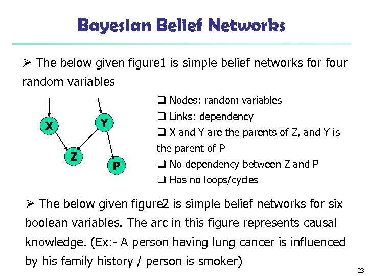
Bayesian Belief Networks Ø The below given figure 1 is simple belief networks for four random variables q Nodes: random variables q Links: dependency Y X Z q X and Y are the parents of Z, and Y is the parent of P P q No dependency between Z and P q Has no loops/cycles Ø The below given figure 2 is simple belief networks for six boolean variables. The arc in this figure represents causal knowledge. (Ex: - A person having lung cancer is influenced by his family history / person is smoker) 23

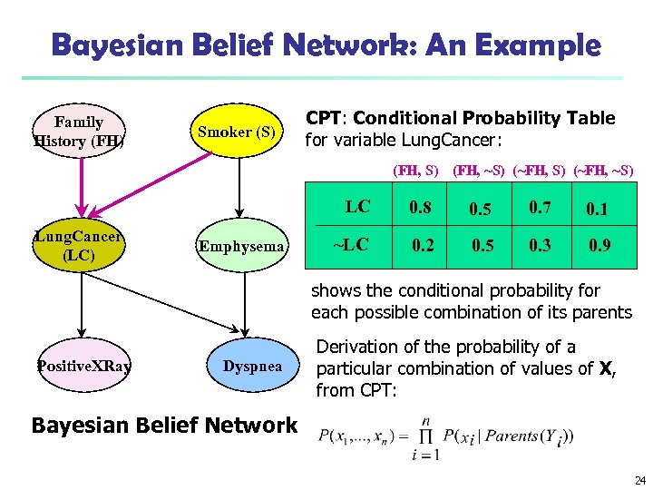
Bayesian Belief Network: An Example Family History (FH) Smoker (S) CPT: Conditional Probability Table for variable Lung. Cancer: (FH, S) (FH, ~S) (~FH, ~S) LC Lung. Cancer (LC) Emphysema 0. 8 0. 5 0. 7 0. 1 ~LC 0. 2 0. 5 0. 3 0. 9 shows the conditional probability for each possible combination of its parents Positive. XRay Dyspnea Derivation of the probability of a particular combination of values of X, from CPT: Bayesian Belief Network 24

Using IF-THEN Rules for Classification n n Rule based classifier make use of a set of IF-THEN rules for classification. We can express a rule of the form, r : (condition) -> y LHS - called as rule antecedent (or) precondition RHS - called as rule consequent Rule set can be expressed as, R = { r 1, r 2, r 3, ……. . , rn } Simply, it represent the knowledge in the form of IF-THEN rules Ex: - n R: IF age = youth AND student = yes THEN buys_computer = yes (or) R: ((age = youth) ^ (student = yes)) -> buys_computer = yes If the condition holds true for given tuple , then antecedent is satisfied. 25

Using IF-THEN Rules for Classification n Assessment of a rule: Using coverage and accuracy we can asses the rule. n ncovers = No. of tuples covered by R n ncorrect = No. of tuples correctly classified by R coverage(R) = ncovers /|D| /* D: training data set */ accuracy(R) = ncorrect / coverage Ex: - R : (age > 40) ^ (income = medium) -> buys_computer=yes ncovers = 3 (the tuples covered by R) ncorrect = 2 (the tuples correctly classified by R) coverage(R) = 3/14 = 0. 214 accuracy(R) = 2/0. 214 = 9. 34 Ø Easy to interpret Ø Easy to generate Ø Can classify new tuples rapidly Ø Highly expensive 26

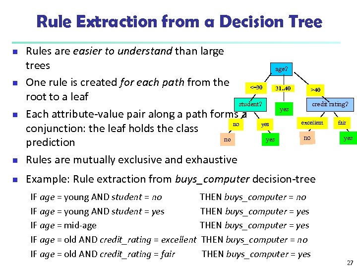
Rule Extraction from a Decision Tree n Rules are easier to understand than large trees age? One rule is created for each path from the <=30 31. . 40 root to a leaf student? yes Each attribute-value pair along a path forms a no yes conjunction: the leaf holds the class no yes prediction Rules are mutually exclusive and exhaustive n Example: Rule extraction from buys_computer decision-tree n n n IF age = young AND student = no IF age = young AND student = yes IF age = mid-age IF age = old AND credit_rating = excellent IF age = old AND credit_rating = fair >40 credit rating? excellent no THEN buys_computer = yes THEN buys_computer = no THEN buys_computer = yes fair yes 27

Classification by Backpropagation n n Back propagation is a neural network learning algorithm. Learning is the process of modifying the weights in order to produce a network that performs some function. Started by psychologists and neurobiologists to develop and test computational analogues of neurons A neural network is a set of connected input/output units where each connection has a weight associated with it During the learning phase, the network learns by adjusting the weights so as to be able to predict the correct class label of the input tuples Many neural network Algorithms existed. One of the popular algorithm is back propagation and it performs learning on multilayer 28

Neural Network as a Classifier n Weakness n n Long training time Require a number of parameters typically best determined empirically, e. g. , the network topology or “structure. ” Poor interpretability: Difficult to interpret the symbolic meaning behind the learned weights and of “hidden units” in the network Strength n High tolerance to noisy data n Ability to classify untrained patterns n Well-suited for continuous-valued inputs and outputs n Successful on an array of real-world data, e. g. , hand-written letters n Algorithms are inherently parallel n Techniques have recently been developed for the extraction of rules from trained neural networks 29

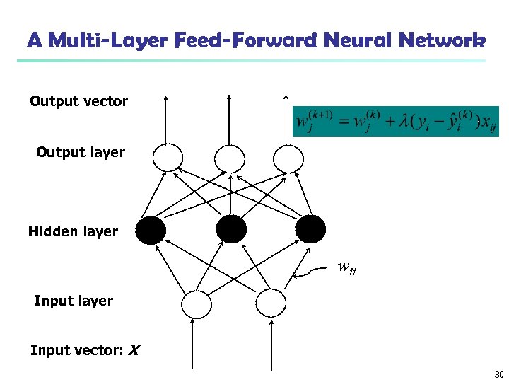
A Multi-Layer Feed-Forward Neural Network Output vector Output layer Hidden layer wij Input layer Input vector: X 30

How A Multi-Layer Neural Network Works n Each layer is made up of units. The inputs to the network correspond to the attributes measured for each training tuple. n Inputs are fed simultaneously into the units making up the input layer n They are then weighted and fed simultaneously to a hidden layer n The number of hidden layers is arbitrary, although usually one n n n The weighted outputs of the last hidden layer are input to units making up the output layer, which emits the network's prediction The units of input layer called as i/p units and output layer called as o/p units and hidden layer units called as neurodes. The network is feed-forward: None of the weights cycles back to an input unit or to an output unit of a previous layer 31

Defining a Network Topology n n n Decide the network topology: Specify # of units in the input layer, # of hidden layers (if > 1), # of units in each hidden layer, and # of units in the output layer Normalize the input values for each attribute measured in the training tuples to [0. 0— 1. 0] One input unit per domain value, each initialized to 0 Output, if for classification and more than two classes, one output unit per class is used Once a network has been trained and its accuracy is unacceptable, repeat the training process with a different network topology or a different set of initial weights 32

Backpropagation n Back propagation learns by Iteratively processing a set of training tuples & compare the network's prediction for each tuple with the actual known target value. (categorical/continuous values) n For each training tuple, the weights are modified to minimize the mean squared error between the network's prediction and the actual target value n Modifications are made in the “backwards” direction: from the output layer, through each hidden layer down to the first hidden layer, hence “backpropagation” n Steps n Initialize weights to small random numbers, associated with biases n Propagate the inputs forward (by applying activation function) n Backpropagate the error (by updating weights and biases) n Terminating condition (when error is very small, etc. ) 33

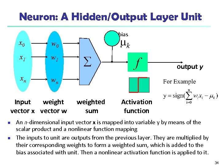
Neuron: A Hidden/Output Layer Unit bias x 0 x 1 w 1 xn wn Input weight vector x vector w n n mk w 0 å weighted sum f output y Activation function An n-dimensional input vector x is mapped into variable y by means of the scalar product and a nonlinear function mapping The inputs to unit are outputs from the previous layer. They are multiplied by their corresponding weights to form a weighted sum, which is added to the bias associated with unit. Then a nonlinear activation function is applied to it. 34

SVM—History and Applications n Vapnik and colleagues (1992)—groundwork from Vapnik & Chervonenkis’ statistical learning theory in 1960 s n Features: training can be slow but accuracy is high owing to their ability to model complex nonlinear decision boundaries (margin maximization) n Used for: classification and numeric prediction n Applications: n handwritten digit recognition, object recognition, speaker identification, benchmarking time-series prediction tests 35

SVM—Support Vector Machines n n n A relatively new classification method for both linear and nonlinear data A support vector machine is an algorithm that works as follows. It uses a nonlinear mapping to transform the original training data into a higher dimension With the new dimension, it searches for the linear optimal separating hyperplane (i. e. , “decision boundary” separating the tuples of one class from another) With an appropriate nonlinear mapping to a sufficiently high dimension, data from two classes can always be separated by a hyperplane SVM finds this hyperplane using support vectors (“essential” training tuples) and margins (defined by the support vectors) 36

Support Vector Machines SVM — When Data Is Linearly Separable ØLet data D be (X 1, y 1), …, (X|D|, y|D|), where Xi is the set of training tuples associated with the class labels yi. Each yi can take one of two values, either +1 or -1 corresponding to the classes buys computer = yes and buys computer = no, respectively. Ø There are infinite lines (hyperplanes) separating the two classes but we want to find the best one (the one that minimizes classification error on unseen data). SVM searches for the hyperplane with the largest margin, i. e. , maximum marginal hyperplane (MMH). Ø Ex: - consider an example based on two input attributes, A 1 and A 2, as shown in Figure. From the graph, we see that the 2 -D data are linearly separable (or “linear, ” ) bz a straight line can be drawn to separate all of the tuples of class +1 from all of the tuples of class -1. 37

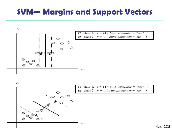
SVM— Margins and Support Vectors Data Mining: Concepts and Techniques 15 March 2018 38

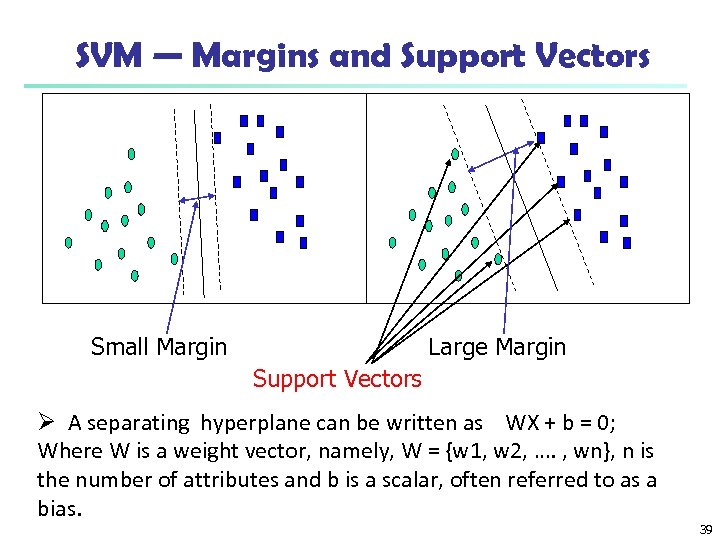
SVM — Margins and Support Vectors Small Margin Large Margin Support Vectors Ø A separating hyperplane can be written as WX + b = 0; Where W is a weight vector, namely, W = {w 1, w 2, …. , wn}, n is the number of attributes and b is a scalar, often referred to as a bias. 39

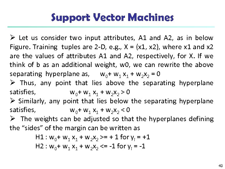
Support Vector Machines Ø Let us consider two input attributes, A 1 and A 2, as in below Figure. Training tuples are 2 -D, e. g. , X = (x 1, x 2), where x 1 and x 2 are the values of attributes A 1 and A 2, respectively, for X. If we think of b as an additional weight, w 0, we can rewrite the above separating hyperplane as, w 0+ w 1 x 1 + w 2 x 2 = 0 Ø Thus, any point that lies above the separating hyperplane satisfies, w 0 + w 1 x 1 + w 2 x 2 > 0 Ø Similarly, any point that lies below the separating hyperplane satisfies, w 0 + w 1 x 1 + w 2 x 2 < 0 Ø The weights can be adjusted so that the hyperplanes defining the “sides” of the margin can be written as H 1 : w 0+ w 1 x 1 + w 2 x 2 >= + 1 for yi = +1 H 2 : w 0+ w 1 x 1 + w 2 x 2 <= -1 for yi = -1 40

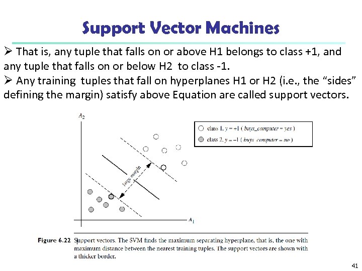
Support Vector Machines Ø That is, any tuple that falls on or above H 1 belongs to class +1, and any tuple that falls on or below H 2 to class -1. Ø Any training tuples that fall on hyperplanes H 1 or H 2 (i. e. , the “sides” defining the margin) satisfy above Equation are called support vectors. 41

Associative Classification n Associative classification: Major steps n Mine data to find strong associations between frequent patterns (conjunctions of attribute-value pairs) and class labels n Association rules are generated in the form of P 1 ^ p 2 … ^ pl “Aclass = C” (conf, sup) n n Organize the rules to form a rule-based classifier Why effective? n It explores highly confident associations among multiple attributes and may overcome some constraints introduced by decision-tree induction, which considers only one attribute at a time n Associative classification has been found to be often more accurate than some traditional classification methods, such as C 4. 5 42

Typical Associative Classification Methods n CBA (Classification Based on Associations: Liu, Hsu & Ma, KDD’ 98) n Mine possible association rules in the form of n n n Build classifier: Organize rules according to decreasing precedence based on confidence and then support CMAR (Classification based on Multiple Association Rules: Li, Han, Pei, ICDM’ 01) n n Cond-set (a set of attribute-value pairs) class label Classification: Statistical analysis on multiple rules CPAR (Classification based on Predictive Association Rules: Yin & Han, SDM’ 03) n Generation of predictive rules (FOIL-like analysis) but allow covered rules to retain with reduced weight n Prediction using best k rules n High efficiency, accuracy similar to CMAR 43

What Is Prediction? n n (Numerical) prediction is similar to classification n construct a model n use model to predict continuous or ordered value for a given input Prediction is different from classification n Classification refers to predict categorical class label n Prediction models continuous-valued functions Major method for prediction: regression n model the relationship between one or more independent or predictor variables and a dependent or response variable Regression analysis n Linear and multiple regression n Non-linear regression n Other regression methods: generalized linear model, Poisson regression, log-linear models, regression trees 44

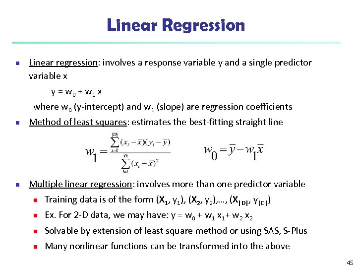
Linear Regression n Linear regression: involves a response variable y and a single predictor variable x y = w 0 + w 1 x where w 0 (y-intercept) and w 1 (slope) are regression coefficients n Method of least squares: estimates the best-fitting straight line n Multiple linear regression: involves more than one predictor variable n Training data is of the form (X 1, y 1), (X 2, y 2), …, (X|D|, y|D|) n Ex. For 2 -D data, we may have: y = w 0 + w 1 x 1+ w 2 x 2 n Solvable by extension of least square method or using SAS, S-Plus n Many nonlinear functions can be transformed into the above 45

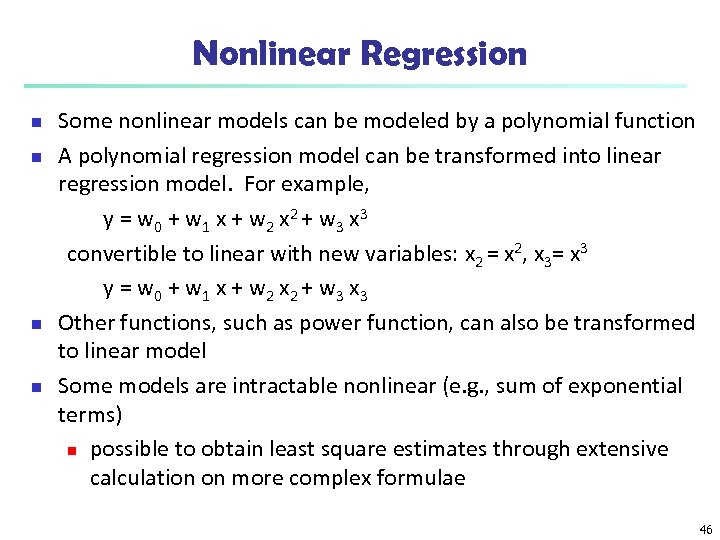
Nonlinear Regression n n Some nonlinear models can be modeled by a polynomial function A polynomial regression model can be transformed into linear regression model. For example, y = w 0 + w 1 x + w 2 x 2 + w 3 x 3 convertible to linear with new variables: x 2 = x 2, x 3= x 3 y = w 0 + w 1 x + w 2 x 2 + w 3 x 3 Other functions, such as power function, can also be transformed to linear model Some models are intractable nonlinear (e. g. , sum of exponential terms) n possible to obtain least square estimates through extensive calculation on more complex formulae 46

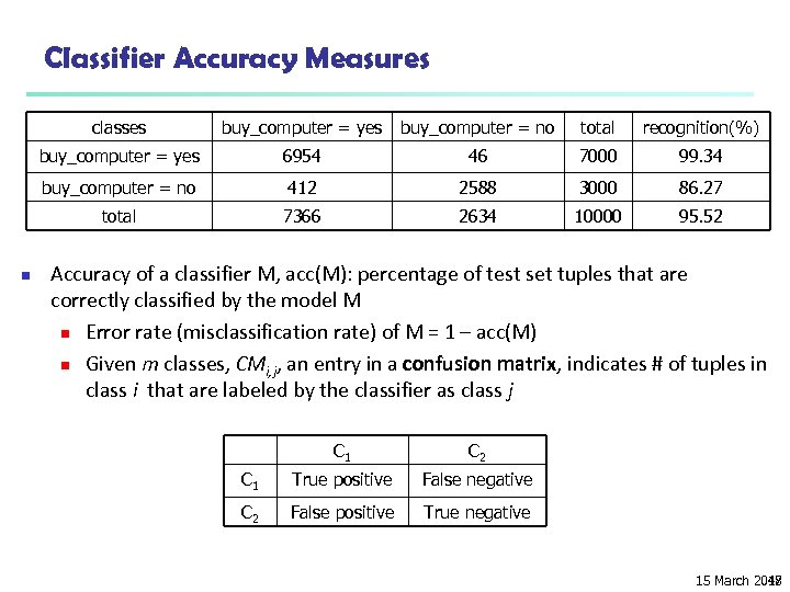
Classifier Accuracy Measures classes buy_computer = no total recognition(%) buy_computer = yes 6954 46 7000 99. 34 buy_computer = no 412 2588 3000 86. 27 total n buy_computer = yes 7366 2634 10000 95. 52 Accuracy of a classifier M, acc(M): percentage of test set tuples that are correctly classified by the model M n Error rate (misclassification rate) of M = 1 – acc(M) n Given m classes, CMi, j, an entry in a confusion matrix, indicates # of tuples in class i that are labeled by the classifier as class j C 1 C 2 C 1 True positive False negative C 2 False positive True negative 15 March 2018 47

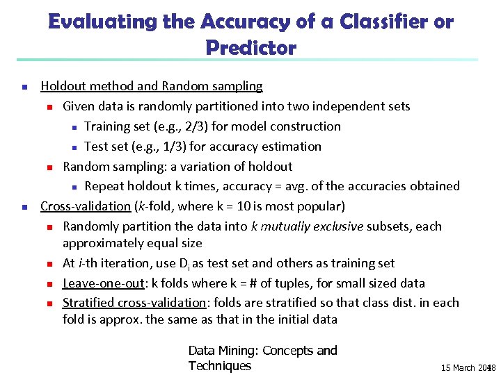
Evaluating the Accuracy of a Classifier or Predictor n n Holdout method and Random sampling n Given data is randomly partitioned into two independent sets n Training set (e. g. , 2/3) for model construction n Test set (e. g. , 1/3) for accuracy estimation n Random sampling: a variation of holdout n Repeat holdout k times, accuracy = avg. of the accuracies obtained Cross-validation (k-fold, where k = 10 is most popular) n Randomly partition the data into k mutually exclusive subsets, each approximately equal size n At i-th iteration, use Di as test set and others as training set n Leave-one-out: k folds where k = # of tuples, for small sized data n Stratified cross-validation: folds are stratified so that class dist. in each fold is approx. the same as that in the initial data Data Mining: Concepts and Techniques 15 March 2018 48

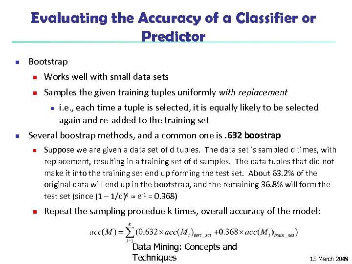
Evaluating the Accuracy of a Classifier or Predictor n Bootstrap n Works well with small data sets n Samples the given training tuples uniformly with replacement n n i. e. , each time a tuple is selected, it is equally likely to be selected again and re-added to the training set Several boostrap methods, and a common one is. 632 boostrap n n Suppose we are given a data set of d tuples. The data set is sampled d times, with replacement, resulting in a training set of d samples. The data tuples that did not make it into the training set end up forming the test set. About 63. 2% of the original data will end up in the bootstrap, and the remaining 36. 8% will form the test set (since (1 – 1/d)d ≈ e-1 = 0. 368) Repeat the sampling procedue k times, overall accuracy of the model: Data Mining: Concepts and Techniques 15 March 2018 49