548cd767938d68caea787bcda4b179da.ppt
- Количество слайдов: 26
 UK FHS Historical sociology (2014+) Quantitative Data Analysis I. & II. Contingency tables: multivariate analysis and elaboration – introduction to 3 -fold of data sorting, ordinal correlations Jiří Šafr jiri. safr(AT)seznam. cz updated 26/11/2014 ® Jiří Šafr, 2014
 Multivariate analysis: threefold level of data sorting in crosstabulation → enables a) more detailed description and b) elaboration (introduction 1. )
 Third level of data sorting in contingency table • A contingency table analysis is used to examine the relationship between two categorical variables (bivariate crosstabulation) • but it can be organized within levels of a third variable. If our goal is elaboration (rather than detailed description), we call it test variable or factor. We aim at to control for its effects. • If a third variable is introduced, it will form separate layers or strata in the table.
 3 rd level of sorting data in contingency table • We analyse simultaneously relationships among several variables (mostly more independent – explanatory variables). • The principle is identical as in bivariate analysis. • The goal of 3 rd level of sorting data is in principle: – More detailed description (in sub/sub-groups) – Elaboration of relationships → searching for causal relations, deeper understanding of context, distinguishing between substantive and false relations, controlling for effect of the 3 rd variable (X↔Y / Z) • This is true also for any 3 rd level of sorting data in general, i. e. also for means in subgroups and linear association (scatter-plots, correlation, regression). We will explain it on contingency tables first.
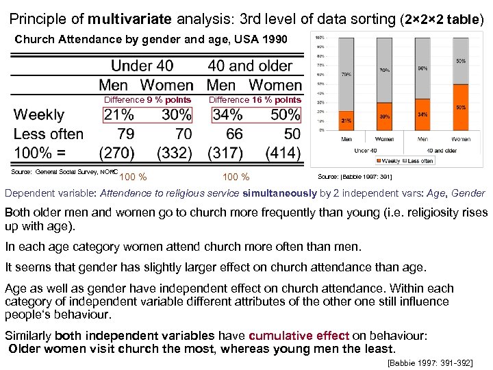 Principle of multivariate analysis: 3 rd level of data sorting (2× 2× 2 table) Church Attendance by gender and age, USA 1990 Difference 9 % points Source: General Social Survey, NORC 100 % Difference 16 % points 100 % Source: [Babbie 1997: 391] Dependent variable: Attendance to religious service simultaneously by 2 independent vars: Age, Gender Both older men and women go to church more frequently than young (i. e. religiosity rises up with age). In each age category women attend church more often than men. It seems that gender has slightly larger effect on church attendance than age. Age as well as gender have independent effect on church attendance. Within each category of independent variable different attributes of the other one still influence people‘s behaviour. Similarly both independent variables have cumulative effect on behaviour: Older women visit church the most, whereas young men the least. [Babbie 1997: 391 -392]
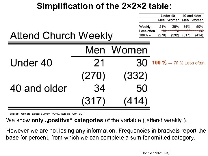 Simplification of the 2× 2× 2 table: 100 % → 70 % Less often Source: General Social Survey, NORC [Babbie 1997: 391] We show only „positive“ categories of the variable („attend weekly“). However we are not losing any information. Frequencies in brackets report the base for percent, from which we can complete a sum for omitted category. [Babbie 1997: 391]
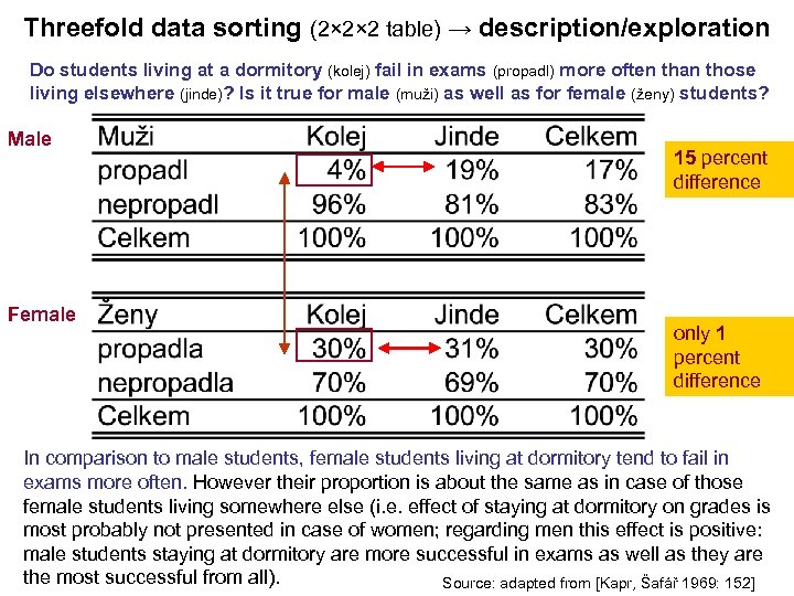 Threefold data sorting (2× 2× 2 table) → description/exploration Do students living at a dormitory (kolej) fail in exams (propadl) more often than those Propadají více studenti „kolejáci“ – as well as for female (ženy) students? living elsewhere (jinde)? Is it true for male (muži)muži nebo „kolejáci“ – ženy? Male Female 15 percent difference only 1 percent difference In comparison to male students, female students living at dormitory tend to fail in exams more often. However their proportion is about the same as in case of those female students living somewhere else (i. e. effect of staying at dormitory on grades is most probably not presented in case of women; regarding men this effect is positive: male students staying at dormitory are more successful in exams as well as they are the most successful from all). Source: adapted from [Kapr, Šafář 1969: 152]
 Introduction into elaboration Threefold data sorting → Controlling for the factor
 Testing / controlling effect of 3 rd variable - factor → Elaboration • Constructing separated tables split by categories of the third variable makes the tested factor holding constant. → relationship between two variables is net – cleaned of distorting effect of this factor variable.
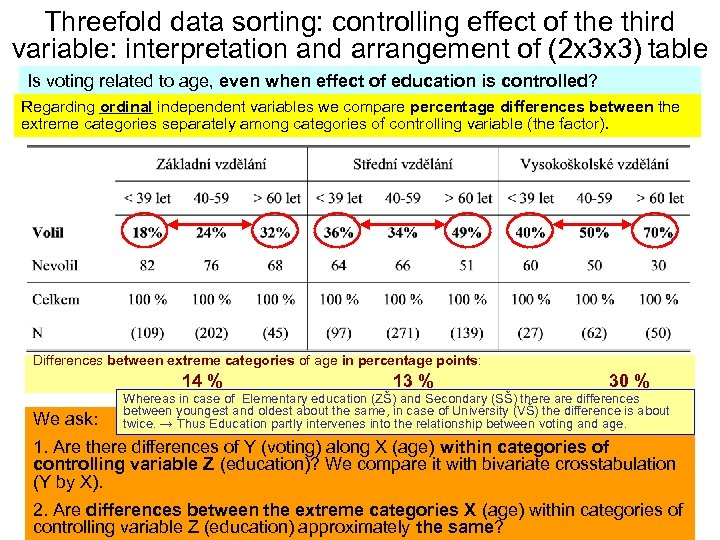 Threefold data sorting: controlling effect of the third variable: interpretation and arrangement of (2 x 3 x 3) table Is voting related to age, even when effect of education is controlled? Regarding ordinal independent variables we compare percentage differences between the extreme categories separately among categories of controlling variable (the factor). Differences between extreme categories of age in percentage points: 14 % We ask: 13 % 30 % Whereas in case of Elementary education (ZŠ) and Secondary (SŠ) there are differences between youngest and oldest about the same, in case of University (VŠ) the difference is about twice. → Thus Education partly intervenes into the relationship between voting and age. 1. Are there differences of Y (voting) along X (age) within categories of controlling variable Z (education)? We compare it with bivariate crosstabulation (Y by X). 2. Are differences between the extreme categories X (age) within categories of controlling variable Z (education) approximately the same?
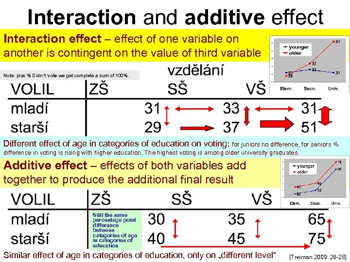 Interaction and additive effect Interaction effect – effect of one variable on another is contingent on the value of third variable Note: plus % Didn‘t vote we get complete a sum of 100%. Different effect of age in categories of education on voting: for juniors no difference, for seniors % difference in voting is rising with higher education. The highest voting is among older university graduates. Additive effect – effects of both variables add together to produce the additional final result Still the same percentage point difference between categories of age in categories of education Similar effect of age in categories of education, only on „different level“ [Treiman 2009: 26 -28]
 Testing the effect of further factor (then in bivariate relationship) • We compare intensity of relationship in original bivariate table with relationships in new tables with third variable-controlling factor (now split into its categories). • If in new tables the association between original variables disappears or is substantially weaken → the association in the original (bivariate) table is function of the third variable (controlling factor) • Further you will see, how to detect hidden relationship quickly using association coefficients within subgroups of the third controlling factor (for nominal variables Phi, Cram. V, Lambda, and ordinal correlation). • Later in QDA II. We will also learn how to standardize (weight) the table along the controlling factor Z, i. e. as if all cases in categories of variable X have the same proportion within categories of Z (e. g. the same education).
 Why we conduct elaboration? 1. To detect and describe interaction (additive) effects and when doing this we can reveal 2. Spurious association (false association/correlation) 3. Suppressed – hidden association The aim is net relationship between two variables when controlled for effect of 3 rd variable. Following two examples will explain it. Coefficients of association (e. g. Lambda used here) are explained in later or in 3. Contingency tables and analysis of categorical data.
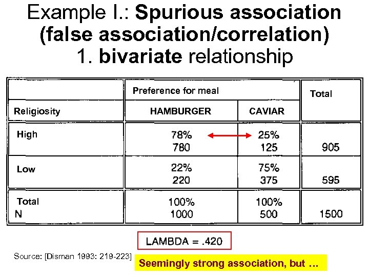 Example I. : Spurious association (false association/correlation) 1. bivariate relationship Preference for meal Religiosity HAMBURGER Total CAVIAR High Low Total Source: [Disman 1993: 219 -223] Seemingly strong association, but …
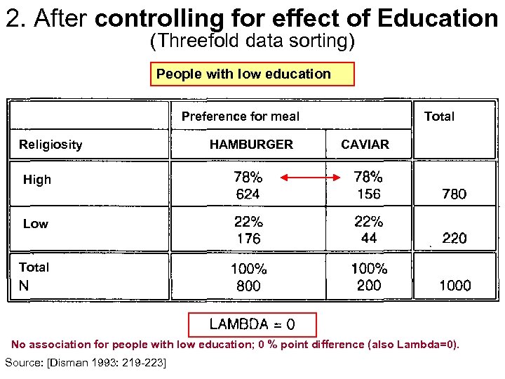 2. After controlling for effect of Education (Threefold data sorting) People with low education Preference for meal Religiosity HAMBURGER Total CAVIAR High Low Total No association for people with low education; 0 % point difference (also Lambda=0). Source: [Disman 1993: 219 -223]
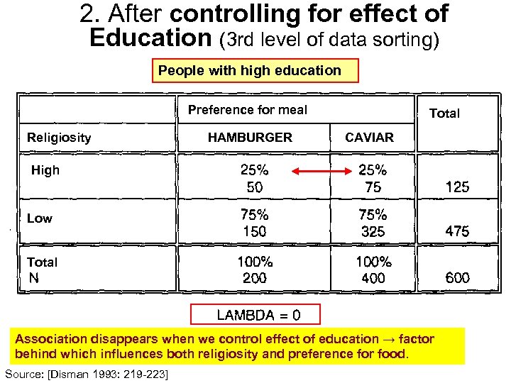 2. After controlling for effect of Education (3 rd level of data sorting) People with high education Preference for meal Religiosity HAMBURGER Total CAVIAR High Low Total Association disappears when we control effect of education → factor behind which influences both religiosity and preference for food. Source: [Disman 1993: 219 -223]
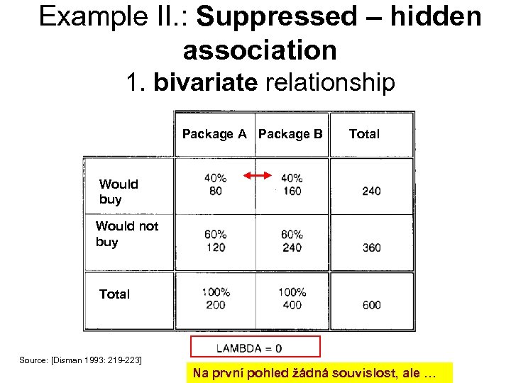 Example II. : Suppressed – hidden association 1. bivariate relationship Package A Package B Total Would buy Would not buy Total Source: [Disman 1993: 219 -223] Na první pohled žádná souvislost, ale …
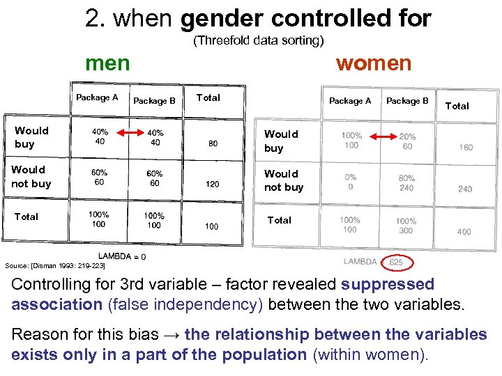 2. when gender controlled for (Threefold data sorting) men Package A women Package B Total Package A Would buy Total Would buy Would not buy Package B Would not buy Total Source: [Disman 1993: 219 -223] Controlling for 3 rd variable – factor revealed suppressed association (false independency) between the two variables. Reason for this bias → the relationship between the variables exists only in a part of the population (within women).
 When examining relationships in elaboration coefficients of association/ordinal correlation can help us find interaction or suppressed effects
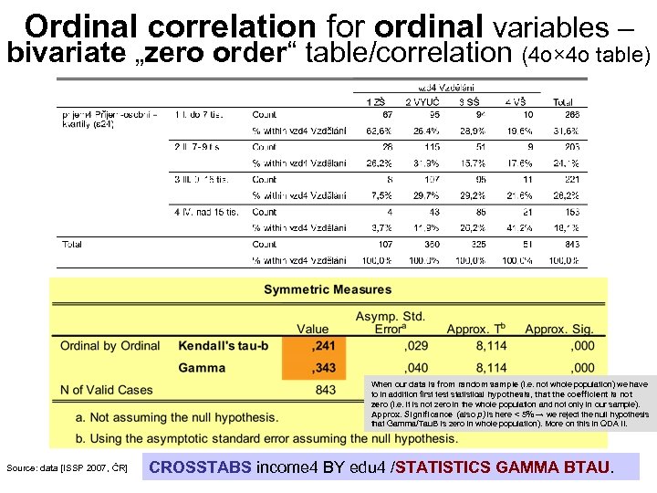 Ordinal correlation for ordinal variables – bivariate „zero order“ table/correlation (4 o× 4 o table) When our data is from random sample (i. e. not whole population) we have to in addition first test statistical hypothesis, that the coefficient is not zero (i. e. it is not zero in the whole population and not only in our sample). Approx. Significance (also p) is here < 5% → we reject the null hypothesis that Gamma/Tau. B is zero in whole population). More on this in QDA II. Source: data [ISSP 2007, ČR] CROSSTABS income 4 BY edu 4 /STATISTICS GAMMA BTAU.
 Is the strength of relationship (ordinal correlation) identical for men and women? → we can compute conditional association/correlation coefficients separately in categories of control variable – factor (gender) Here 4 o× 2 table.
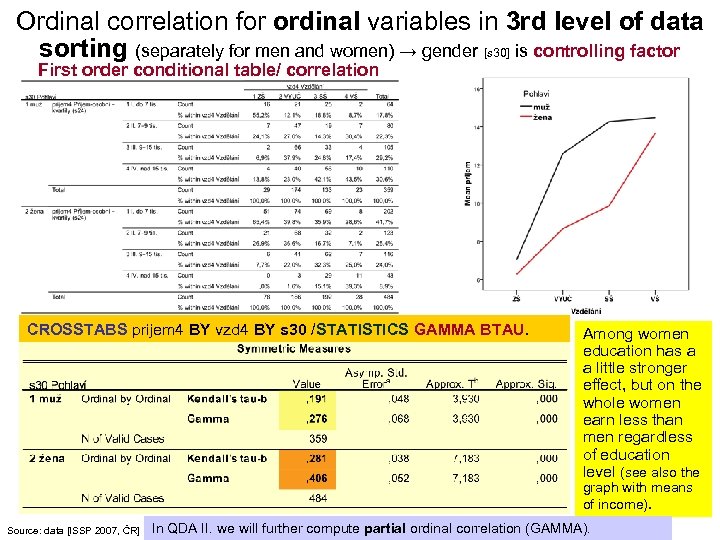 Ordinal correlation for ordinal variables in 3 rd level of data sorting (separately for men and women) → gender [s 30] is controlling factor First order conditional table/ correlation CROSSTABS prijem 4 BY vzd 4 BY s 30 /STATISTICS GAMMA BTAU. Among women education has a a little stronger effect, but on the whole women earn less than men regardless of education level (see also the graph with means of income). Source: data [ISSP 2007, ČR] In QDA II. we will further compute partial ordinal correlation (GAMMA).
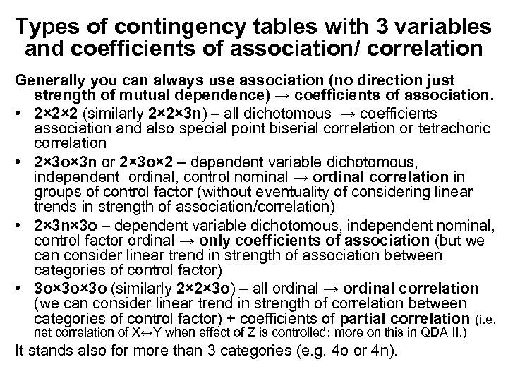 Types of contingency tables with 3 variables and coefficients of association/ correlation Generally you can always use association (no direction just strength of mutual dependence) → coefficients of association. • 2× 2× 2 (similarly 2× 2× 3 n) – all dichotomous → coefficients association and also special point biserial correlation or tetrachoric correlation • 2× 3 o× 3 n or 2× 3 o× 2 – dependent variable dichotomous, independent ordinal, control nominal → ordinal correlation in groups of control factor (without eventuality of considering linear trends in strength of association/correlation) • 2× 3 n× 3 o – dependent variable dichotomous, independent nominal, control factor ordinal → only coefficients of association (but we can consider linear trend in strength of association between categories of control factor) • 3 o× 3 o (similarly 2× 2× 3 o) – all ordinal → ordinal correlation (we can consider linear trend in strength of correlation between categories of control factor) + coefficients of partial correlation (i. e. net correlation of X↔Y when effect of Z is controlled; more on this in QDA II. ) It stands also for more than 3 categories (e. g. 4 o or 4 n).
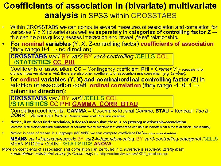 Coefficients of association in (bivariate) multivariate analysis in SPSS within CROSSTABS • Within CROSSTABS we can compute several measures of association and correlation for variables Y x X (bivariate) as well as separately in categories of controlling factor Z → this can help us quickly assess interaction and reveal „false“ relationship. • For nominal variables (Y, X, Z-controlling factor) coefficients of association (they range 0 -1 → no direction): CROSSTABS var 1 BY var 2 BY var 3 -controlling /CELLS COL /STATISTICS CC PHI. Coefficients of association: CC = Contingency coefficient, PHI = Cramer V (+ equivalent for dichotomised variables is Phi); there also other coefficients of association and correlation (e. g. Lambda). • for ordinal variables (Y, X) and nominal/ordinal controlling factor (Z) in addition of association coeff. ordinal correlation (they range -1– 0– 1 → determine direction): CROSSTABS var 1 BY var 2 /CELLS COL /STATISTICS CC PHI GAMMA CORR BTAU. Correlation coefficients: GAMMA = Goodman&Kruskal Gamma, BTAU = Kendaull Tau B, CORR = Spearman Rho (+ Pearson correl. coef. R for ratio variables) • Notice, if we don‘t find correlation, it doesn't mean that, there is no (strong) relationship–association. Moreover with ordinal variables comparison of correlations and coefficients of association can help us indicate what is the relationship (nonlinearity). • Notice: in case of means in subgroups (MEANS) we van compute coefficient Eta 2 (for ratio x nominal variable) : MEANS var 1 -dependet-numeric BY var 2 -independent-categ. BY var 3 -controlling-categorial /CELLS MEAN STDDEV COUNT /STATISTICS ANOVA. More on coeficients of association and correlation can be found in 2. Korelace a asociace: vztahy mezi kardinálními/ ordinálními znaky (in Czech only) na http: //metodykv. wz. cz/AKD 2_korelace. ppt
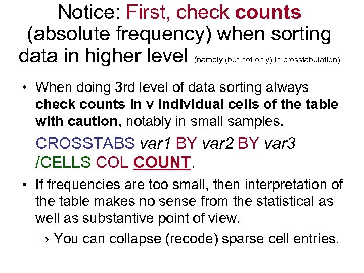 Notice: First, check counts (absolute frequency) when sorting data in higher level (namely (but not only) in crosstabulation) • When doing 3 rd level of data sorting always check counts in v individual cells of the table with caution, notably in small samples. CROSSTABS var 1 BY var 2 BY var 3 /CELLS COL COUNT. • If frequencies are too small, then interpretation of the table makes no sense from the statistical as well as substantive point of view. → You can collapse (recode) sparse cell entries.
 More examples will be added later …


