Types of Market Structure Pure Competition or

Types of Market Structure • Pure Competition or Perfect Competition • Monopoly • Monopolistic Competition • Oligopoly

Perfect Competition

Assumptions of Perfect Competition • Many independent firms • Each seller is small relative to the whole market • Homogeneous (identical) product • Easy entry and exit (no barriers to entry)

Price Taking The perfectly competitive firm is said to be a price-taker, because it takes the market price as given and has no control over the price. Why? . . .

If the firm tried to charge a higher price, it would lose all its business. Customers could go elsewhere to buy the same product for less. Since the firm is very small, it can sell as much as it wants at the market price. So there’s no reason to charge a lower price.

The demand curve for the product of the perfectly competitive firm shows how much can be sold at specific prices. Let’s see what it would look like. . . The firm can sell as little or as much as it wants at the market price. Suppose, for example, the market price is $5.

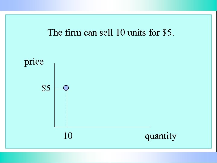The firm can sell 10 units for $5. price $5 10 quantity

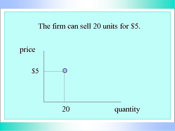The firm can sell 20 units for $5. price $5 20 quantity

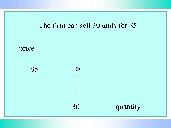The firm can sell 30 units for $5. price $5 30 quantity

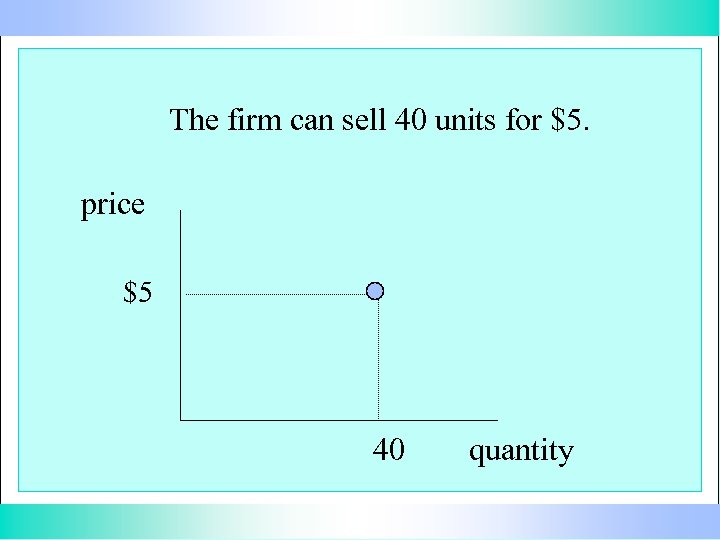The firm can sell 40 units for $5. price $5 40 quantity

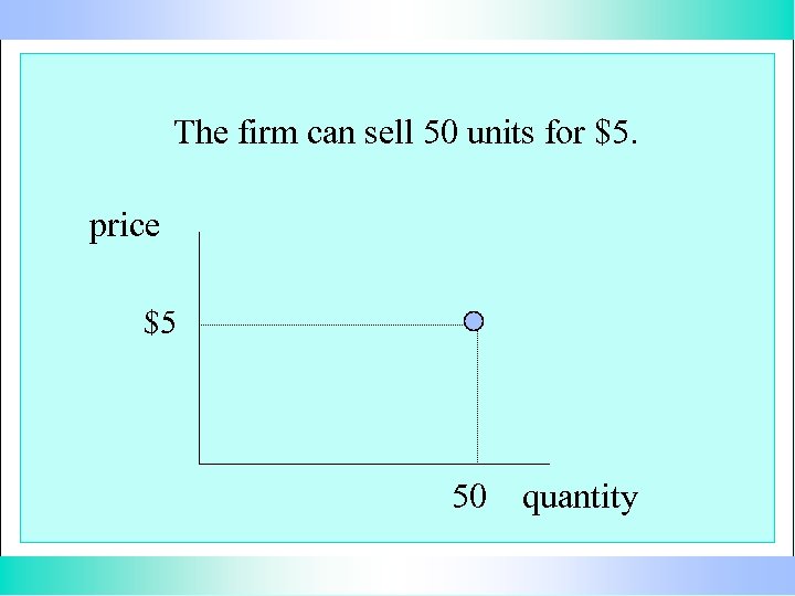The firm can sell 50 units for $5. price $5 50 quantity

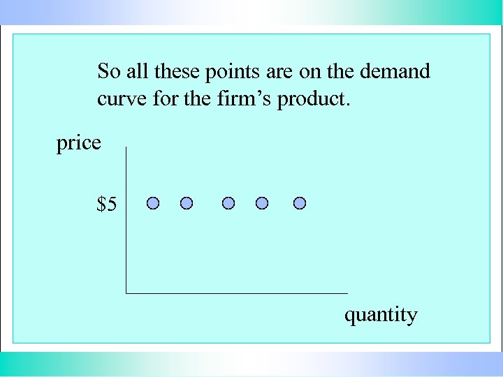So all these points are on the demand curve for the firm’s product. price $5 quantity

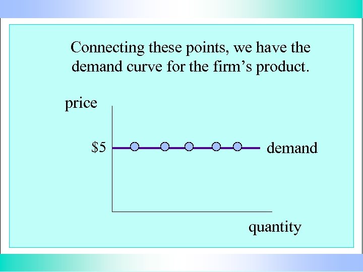Connecting these points, we have the demand curve for the firm’s product. price $5 demand quantity

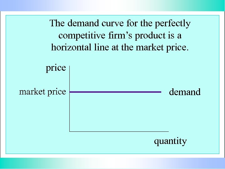The demand curve for the perfectly competitive firm’s product is a horizontal line at the market price demand quantity

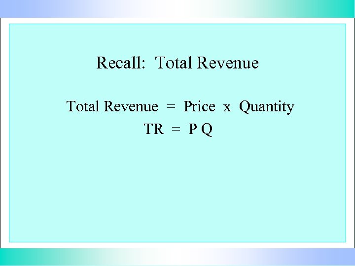Recall: Total Revenue = Price x Quantity TR = P Q

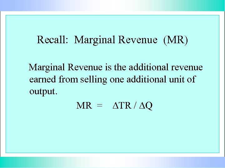Recall: Marginal Revenue (MR) Marginal Revenue is the additional revenue earned from selling one additional unit of output. MR = DTR / DQ

comment For ease of writing, instead of writing the “perfectly competitive” firm we will frequently write the “p. c. ” firm.

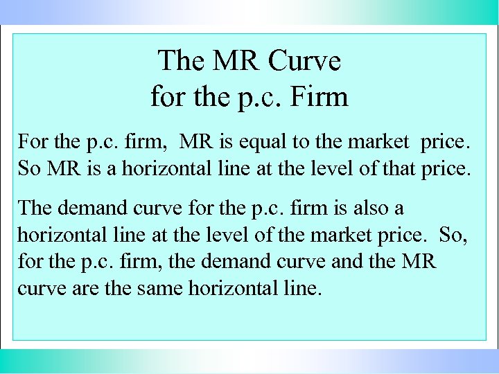The MR Curve for the p. c. Firm For the p. c. firm, MR is equal to the market price. So MR is a horizontal line at the level of that price. The demand curve for the p. c. firm is also a horizontal line at the level of the market price. So, for the p. c. firm, the demand curve and the MR curve are the same horizontal line.

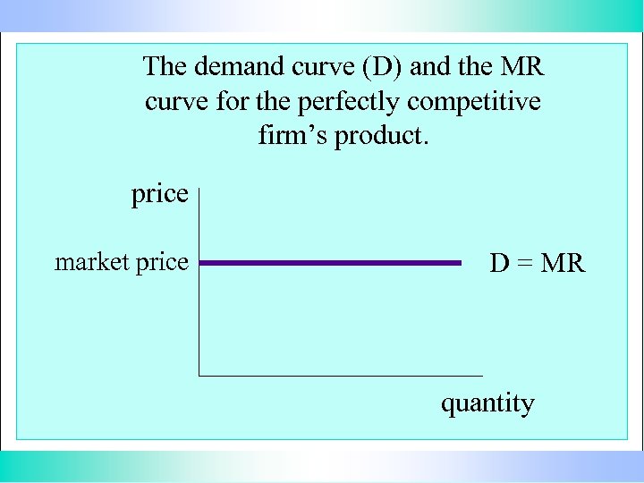The demand curve (D) and the MR curve for the perfectly competitive firm’s product. price market price D = MR quantity

Optimal Output Level Recall: To maximize profit, the firm will produce at the output level where MR = MC. So the firm will produce where the MR and MC curves intersect.

Draw your axes; label them quantity and $. $ Quantity

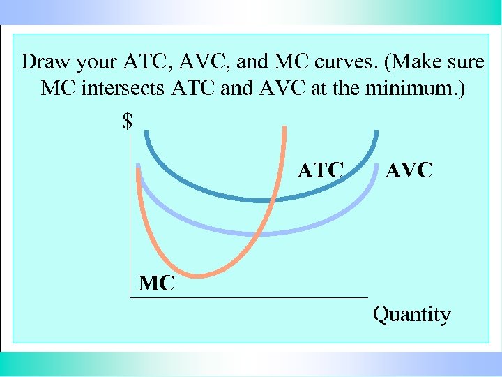Draw your ATC, AVC, and MC curves. (Make sure MC intersects ATC and AVC at the minimum. ) $ ATC AVC MC Quantity

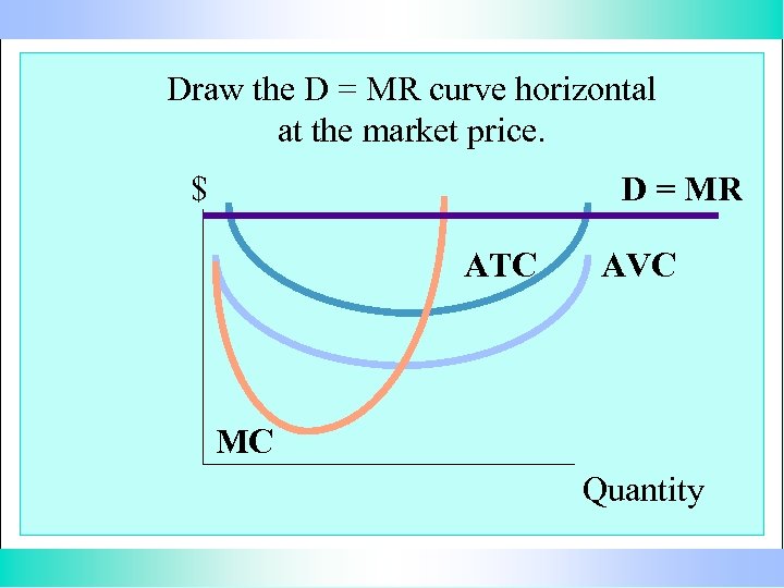Draw the D = MR curve horizontal at the market price. $ D = MR ATC AVC MC Quantity

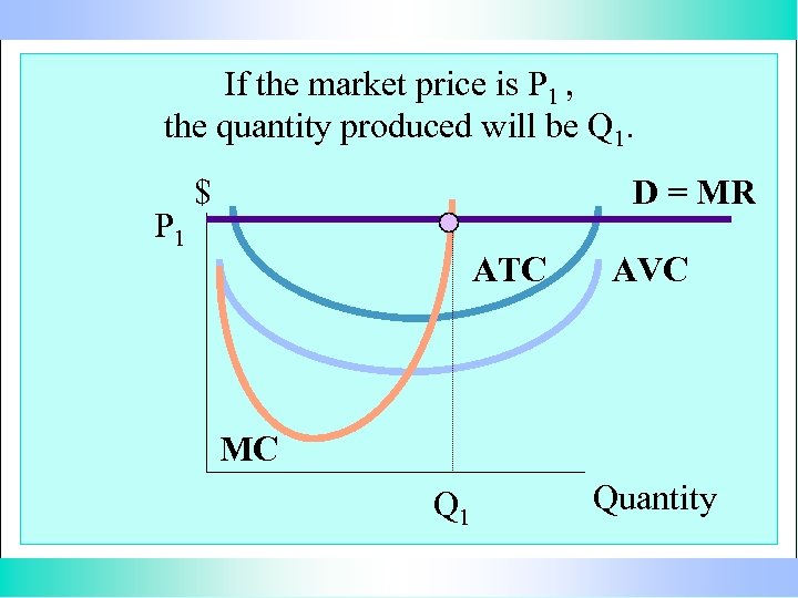If the market price is P 1 , the quantity produced will be Q 1. P 1 $ D = MR ATC AVC MC Q 1 Quantity

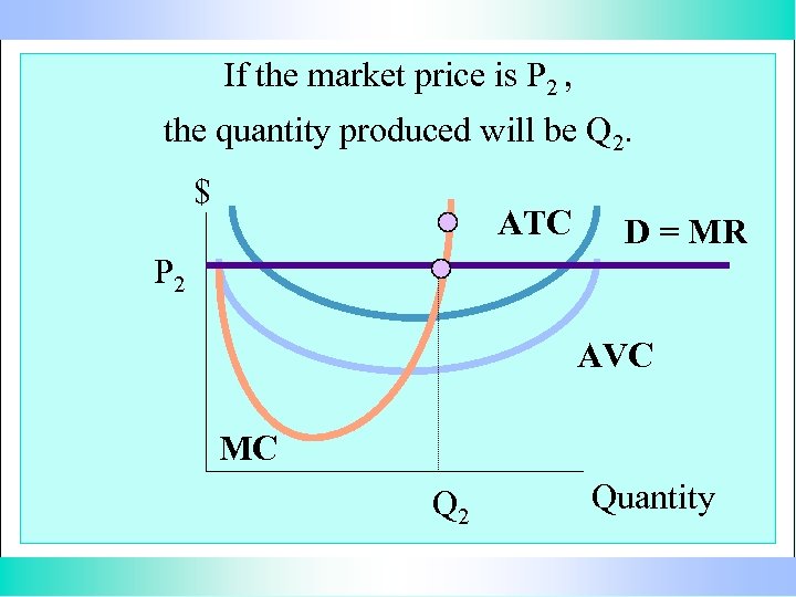If the market price is P 2 , the quantity produced will be Q 2. $ ATC D = MR P 2 AVC MC Q 2 Quantity

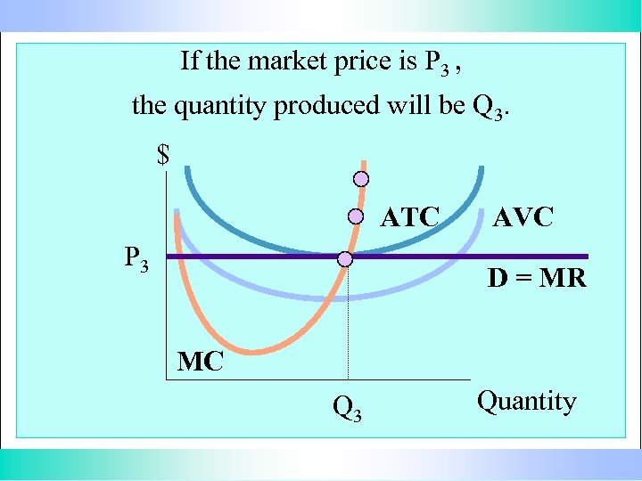If the market price is P 3 , the quantity produced will be Q 3. $ ATC P 3 AVC D = MR MC Q 3 Quantity

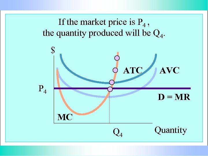If the market price is P 4 , the quantity produced will be Q 4. $ ATC P 4 AVC D = MR MC Q 4 Quantity

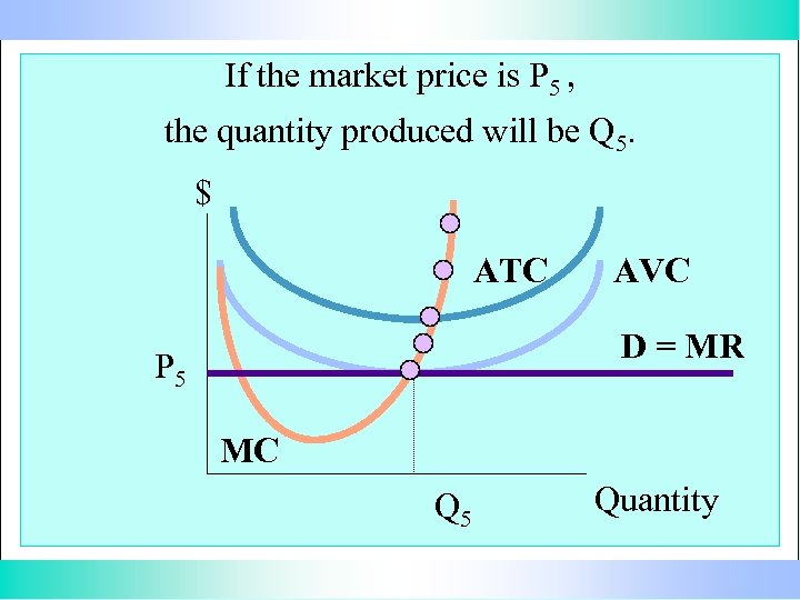If the market price is P 5 , the quantity produced will be Q 5. $ ATC AVC D = MR P 5 MC Q 5 Quantity

Price P 5 was the minimum of the AVC curve (the shutdown point). If the price fell any lower than P 5 the firm would produce no output.

The p. c. firm’s short run supply curve The firm’s supply curve shows the quantity the firm will produce at each price. The P, Q values we have shown, therefore, are points on the firm’s supply curve. But those points are all on the firm’s MC curve. So, the firm’s supply curve is the part of the MC curve that is above the minimum of the AVC curve.

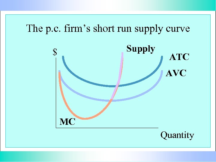The p. c. firm’s short run supply curve Supply $ ATC AVC MC Quantity

The market short run supply curve To determine the total amount that all the firms will produce at each price, we simply add up the amounts that each of the firms will produce at that price.

Graphing Profit

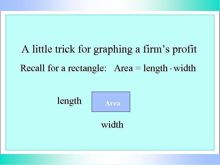A little trick for graphing a firm’s profit Recall for a rectangle: Area = length. width length Area width

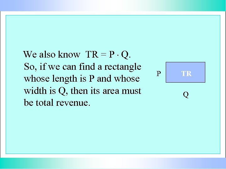We also know TR = P. Q. So, if we can find a rectangle whose length is P and whose width is Q, then its area must be total revenue. P TR Q

To determine Total Cost, first remember ATC = TC / Q So, ATC. Q = TC

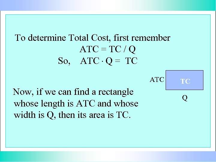To determine Total Cost, first remember ATC = TC / Q So, ATC. Q = TC ATC Now, if we can find a rectangle whose length is ATC and whose width is Q, then its area is TC. TC Q

Then to determine profit, we just subtract the TC area from the TR area.

Graphing Profit: The six steps

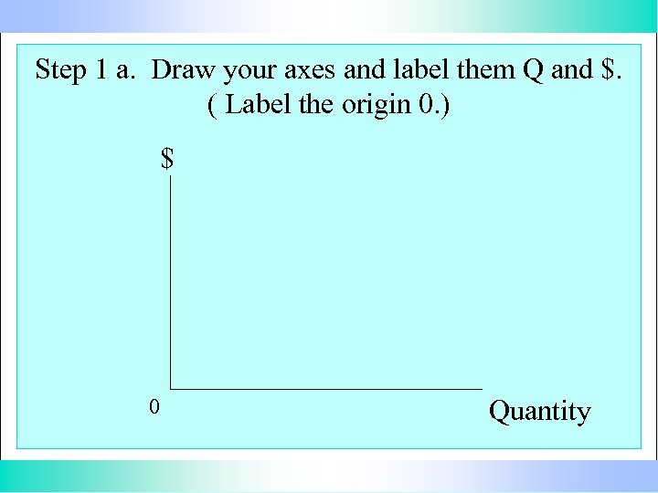Step 1 a. Draw your axes and label them Q and $. ( Label the origin 0. ) $ 0 Quantity

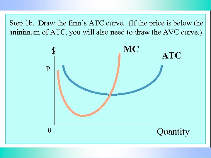Step 1 b. Draw the firm’s ATC curve. (If the price is below the minimum of ATC, you will also need to draw the AVC curve. ) $ MC ATC P 0 Quantity

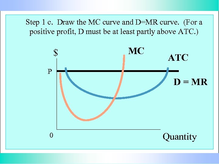Step 1 c. Draw the MC curve and D=MR curve. (For a positive profit, D must be at least partly above ATC. ) $ MC ATC P D = MR 0 Quantity

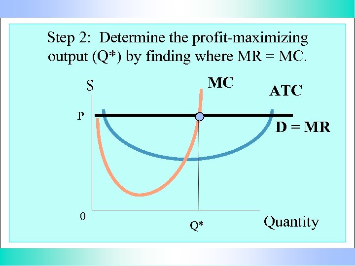Step 2: Determine the profit-maximizing output (Q*) by finding where MR = MC. MC $ P 0 ATC D = MR Q* Quantity

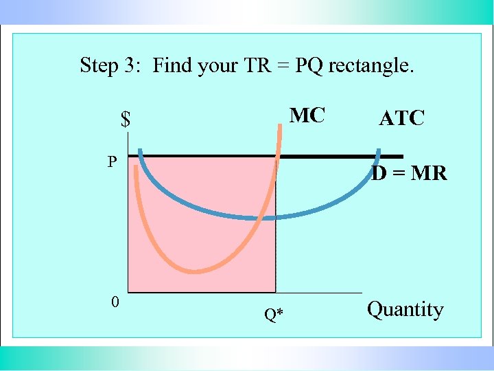Step 3: Find your TR = PQ rectangle. MC $ P 0 ATC D = MR Q* Quantity

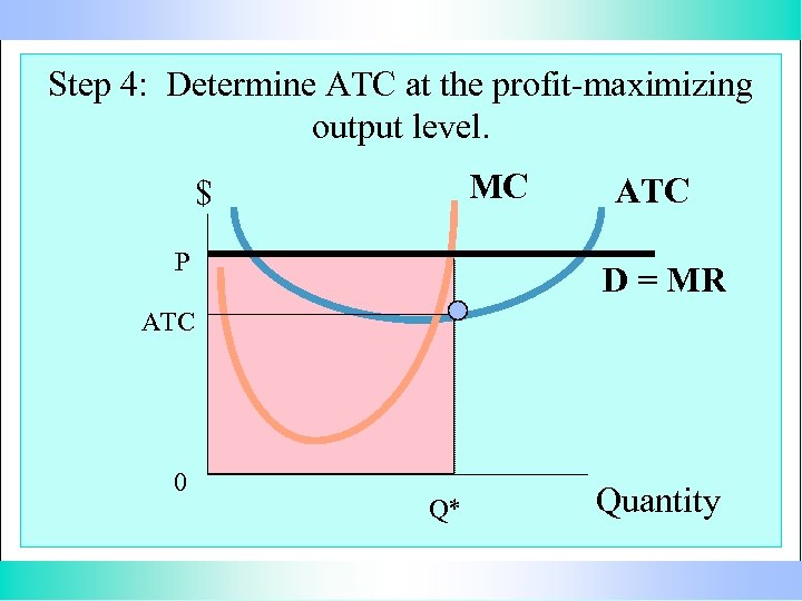Step 4: Determine ATC at the profit-maximizing output level. MC $ P ATC D = MR ATC 0 Q* Quantity

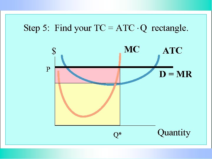Step 5: Find your TC = ATC. Q rectangle. MC $ P ATC D = MR Q* Quantity

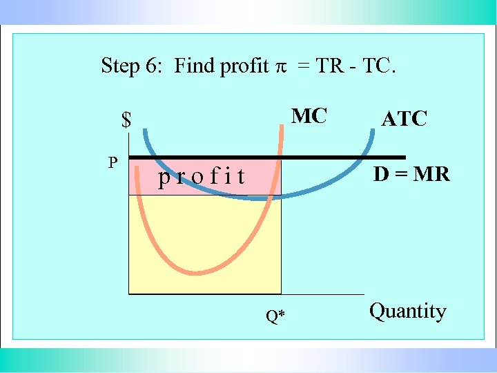Step 6: Find profit p = TR - TC. MC $ P ATC D = MR profit Q* Quantity

You follow the same steps to draw a firm that is making a loss or breaking even (zero profits). Let’s do a firm with a loss.

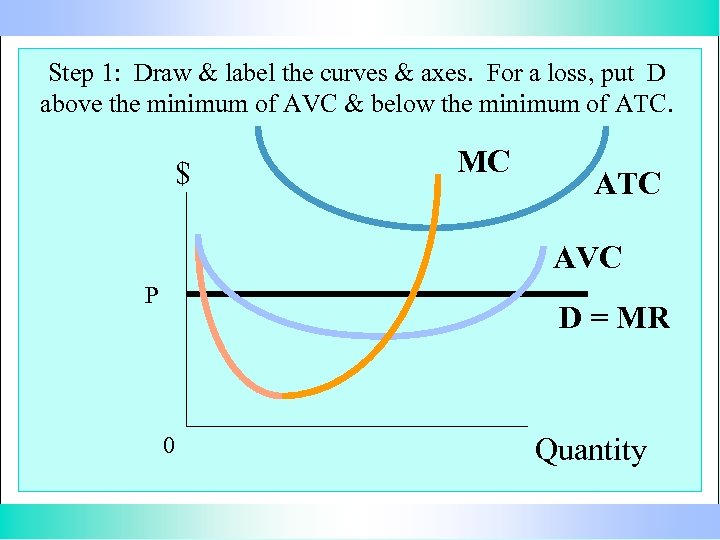Step 1: Draw & label the curves & axes. For a loss, put D above the minimum of AVC & below the minimum of ATC. $ MC ATC AVC P D = MR 0 Quantity

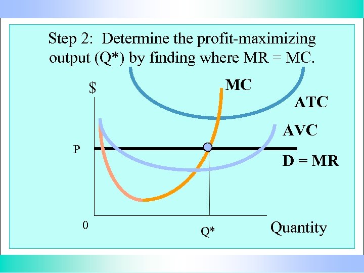Step 2: Determine the profit-maximizing output (Q*) by finding where MR = MC. MC $ ATC AVC P D = MR 0 Q* Quantity

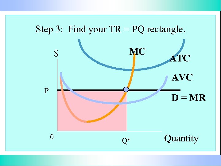Step 3: Find your TR = PQ rectangle. $ MC ATC AVC P D = MR 0 Q* Quantity

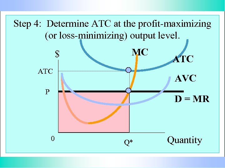Step 4: Determine ATC at the profit-maximizing (or loss-minimizing) output level. $ MC ATC AVC P D = MR 0 Q* Quantity

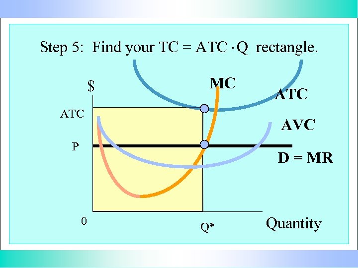Step 5: Find your TC = ATC. Q rectangle. $ MC ATC AVC P D = MR 0 Q* Quantity

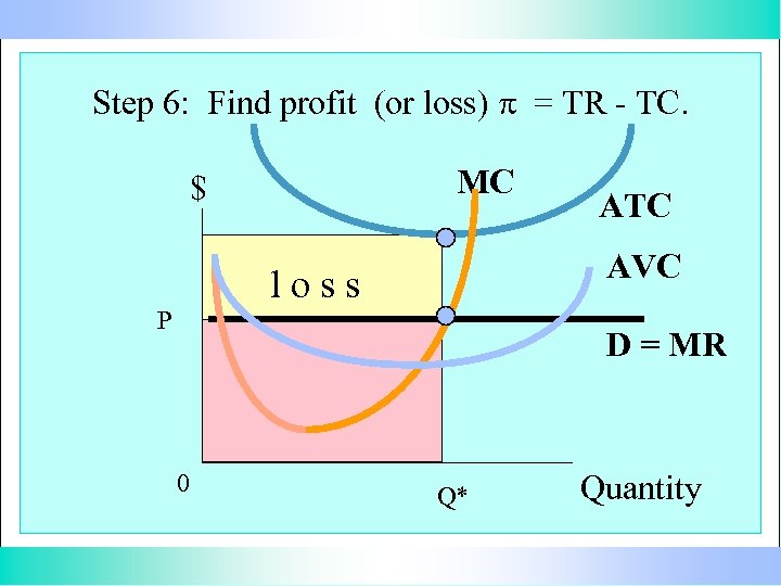Step 6: Find profit (or loss) p = TR - TC. MC $ ATC AVC loss P D = MR 0 Q* Quantity

A firm that is breaking even (zero profits)

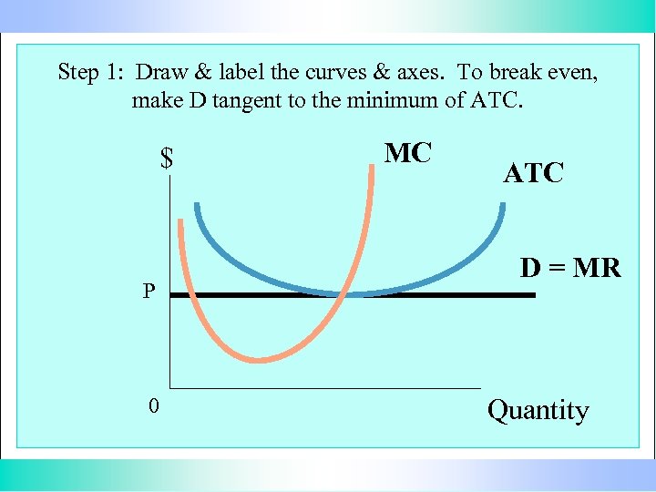Step 1: Draw & label the curves & axes. To break even, make D tangent to the minimum of ATC. $ P 0 MC ATC D = MR Quantity

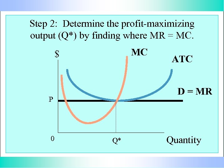Step 2: Determine the profit-maximizing output (Q*) by finding where MR = MC. MC $ D = MR P 0 ATC Q* Quantity

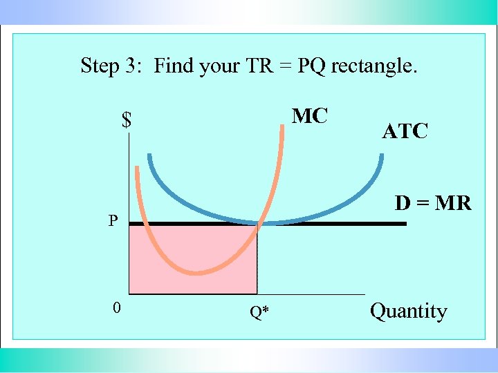Step 3: Find your TR = PQ rectangle. MC $ D = MR P 0 ATC Q* Quantity

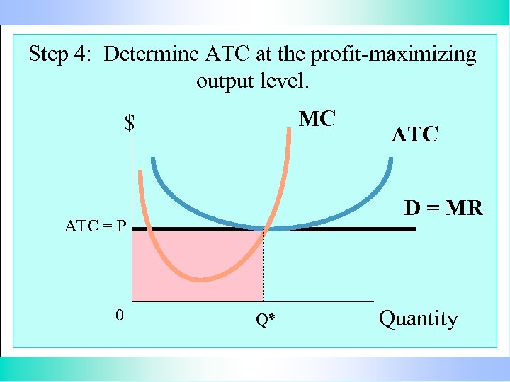Step 4: Determine ATC at the profit-maximizing output level. MC $ D = MR ATC = P 0 ATC Q* Quantity

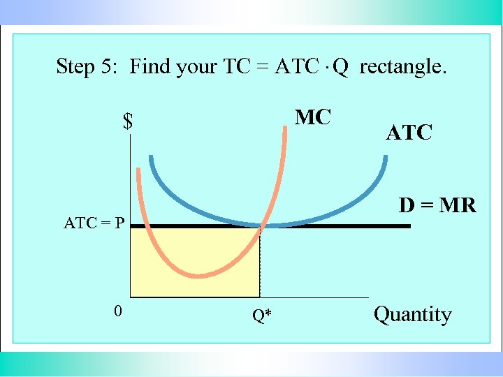Step 5: Find your TC = ATC. Q rectangle. MC $ D = MR ATC = P 0 ATC Q* Quantity

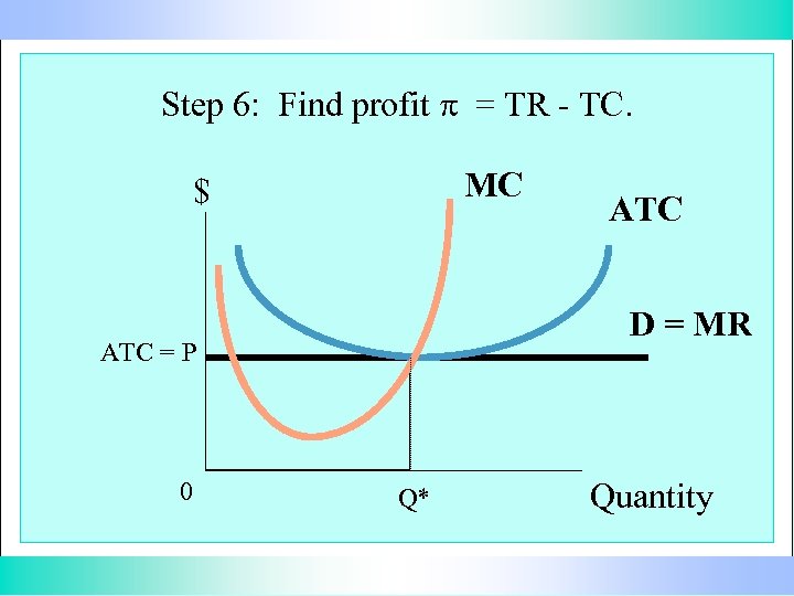Step 6: Find profit p = TR - TC. MC $ D = MR ATC = P 0 ATC Q* Quantity

Adapting to Changes in Demand

Constant Cost Industry an industry in which costs of production remain constant as output in the industry expands

Let’s start with the industry in long run equilibrium. What is each firm’s economic profit (+, – , or 0)? Zero. That means that the price is at the minimum of the ATC curve and is just sufficient to cover the cost per unit of producing the good. Next suppose that demand increases. What happens to the price? It increases.

If firms were just breaking even (zero economic profit) at the old price, what will profit be at the new higher price? It will be positive. Does positive economic profit mean that the firms are doing better, worse, or about the same as firms in other industries are doing? Better. What is the nature of barriers to entry in perfect competition? There are no barriers to entry. So we’ve got positive economic profit and no barriers to entry. What will happen? Firms will enter the industry.

What will happen to the supply of the product as new firms enter the industry? It will increase. What happens to the price of the product? It falls. So the price goes back to where it was before the demand change, but there is more output being produced by more firms. Note that if the price didn’t drop enough, there would still be positive economic profits and firms would continue to enter the industry, supply would keep increasing, and the price would drop some more. If the price dropped too much, it would not cover costs per unit, and there would be losses. Firms would leave the industry, supply would fall and the price would come back up to just covering costs per unit.

So what has happened as a result of the increase in demand in this constant cost industry? We now have the same price we had before, but we now have more output because we have more firms in the industry. So in a constant cost industry, firms will produce as much or as little as the economy demands at a price which is just enough to cover the cost per unit.

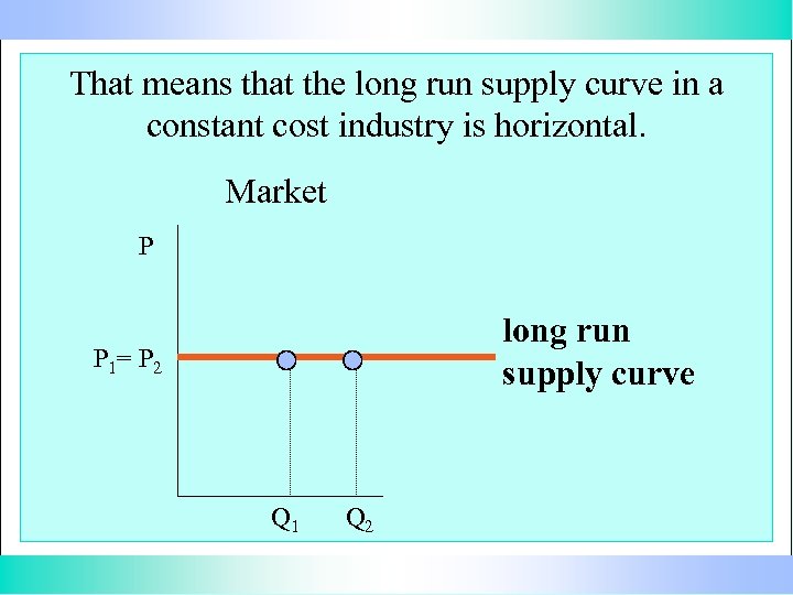That means that the long run supply curve in a constant cost industry is horizontal. Market P long run supply curve P 1= P 2 Q 1 Q 2

Increasing Cost Industry an industry in which costs of production increase as output in the industry expands

Let’s start again with the industry in long run equilibrium. What is each firm’s economic profit (+, – , or 0)? Zero. So the price is at the minimum of the ATC curve and is just sufficient to cover the cost per unit of producing the good. Next suppose that demand increases. What happens to the price? It increases.

If firms were just breaking even (zero economic profit) at the old price, what will happen to profit at the new higher price? It will be positive. Are the firms are doing better, worse, or about the same as firms in other industries are doing? Better. What is the nature of the barriers to entry in perfect competition? There are no barriers to entry. So we’ve got positive economic profit and no barriers to entry. What will happen? Firms will enter the industry.

What will happen to the supply of the product as new firms enter the industry? It will increase. Before when we had a constant cost industry, the costs remained the same as the industry expanded. However, now we have an increasing cost industry. That means that as the industry expands, it puts upward pressure on the price of the inputs used in the industry and the cost of production increases. So visualize all the cost curves, including the ATC, creeping up.

So the industry supply curve is shifting to the right, and the ATC and other cost curves are creeping up. As the supply increases, what happens to the price of the product? It falls. But the price does not fall back to where it was before the demand change, which was at the minimum of the old ATC curve. It only drops until we are back to zero economic profits under the new conditions, which is at the bottom of the new, higher, ATC curve.

So what has happened as a result of the increase in demand in this increasing cost industry? Supply expanded in response to the increased profits resulting from the increase in demand. However, costs increased so that we ended up with a higher price that is just enough to cover the new higher cost per unit.

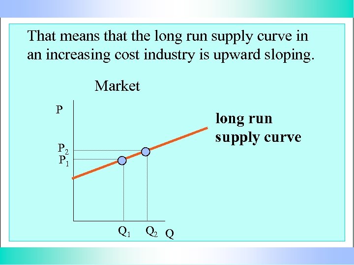That means that the long run supply curve in an increasing cost industry is upward sloping. Market P long run supply curve P 2 P 1 Q 2 Q

Decreasing Cost Industry an industry in which costs of production fall as output in the industry expands

Let’s start again with the industry in long run equilibrium. What is each firm’s economic profit (+, – , or 0)? Zero. So the price is at the minimum of the ATC curve and is just sufficient to cover the cost per unit of producing the good. Next suppose that demand increases. What happens to the price? It increases.

If firms were just breaking even at the old price, what will happen to profit at the new higher price? It will be positive. Are the firms are doing better, worse, or about the same as firms in other industries are doing? Better. What is the nature of the barriers to entry in perfect competition? There are no barriers to entry. So we’ve got positive economic profit and no barriers to entry. What will happen? Firms will enter the industry.

What will happen to the supply of the product as new firms enter the industry? It will increase. Now we have a decreasing cost industry. That means that as the industry expands and infrastructure improves, the cost of production decreases. So visualize all the cost curves, including the ATC, sliding down.

So the industry supply curve is shifting to the right, and the ATC and other cost curves are sliding down. As the supply increases, what happens to the price of the product? It falls. But the price does not fall back to where it was before the demand change, which was at the minimum of the old ATC curve. It keeps dropping until we are back to zero economic profits under the new conditions, which is at the bottom of the new, lower, ATC curve.

So what has happened as a result of the increase in demand in this decreasing cost industry? Supply expanded in response to the increased profits resulting from the increase in demand. However, costs decreased so that we ended up with a lower price that is just enough to cover the new lower cost per unit.

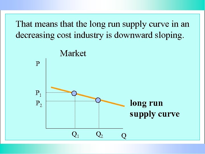That means that the long run supply curve in an decreasing cost industry is downward sloping. Market P P 1 P 2 long run supply curve Q 1 Q 2 Q

Good Things about Perfect Competition • Costs are minimized. Competition forces efficient operation. Inefficient firms will have losses and be forced out of business. • P = MC The price (which comes from the demand curve) is the amount that consumers value a good. MC is the cost of producing an additional unit of a good. So firms produce up to the point where the amount that consumers value a good is equal to the amount it costs to produce an additional unit of the good.