Tutorial Workshop DDSA DISCRETE DYNAMICAL SYSTEMS AND APPLICATONS

Tutorial Workshop DDSA DISCRETE DYNAMICAL SYSTEMS AND APPLICATONS Urbino, June 30 -July 3 March 2010 Closed invariant curves and their bifurcations in two-dimensional maps Anna Agliari Catholic University Via Emilia Parmense, 84. 29100 Piacenza (Italy) anna. agliari@unicatt. it

AIM OF THE LECTURE To show some global bifurcations related to l the appearance/disappearance of closed invariant curves; l the interaction between coexisting cycles and closed invariant curves; SADDLE CONNECTIONS and HOMOCLINIC TANGLES

CONTENTS & & & : INVARIANT SETS HOMOCLINIC AND HETEROCLINIC ORBITS INVARIANT CLOSED CURVES GLOBAL BIFURCATIONS OF INVARIANT CURVES : A PROPEDEUTIC EXAMPLE : A FINANCIAL MARKET MODEL : A BUSINESS CYCLE MODEL

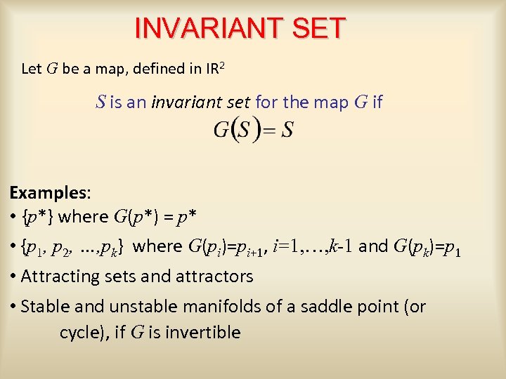INVARIANT SET Let G be a map, defined in IR 2 S is an invariant set for the map G if Examples: • {p*} where G(p*) = p* • {p 1, p 2, …, pk} where G(pi)=pi+1, i=1, …, k-1 and G(pk)=p 1 • Attracting sets and attractors • Stable and unstable manifolds of a saddle point (or cycle), if G is invertible

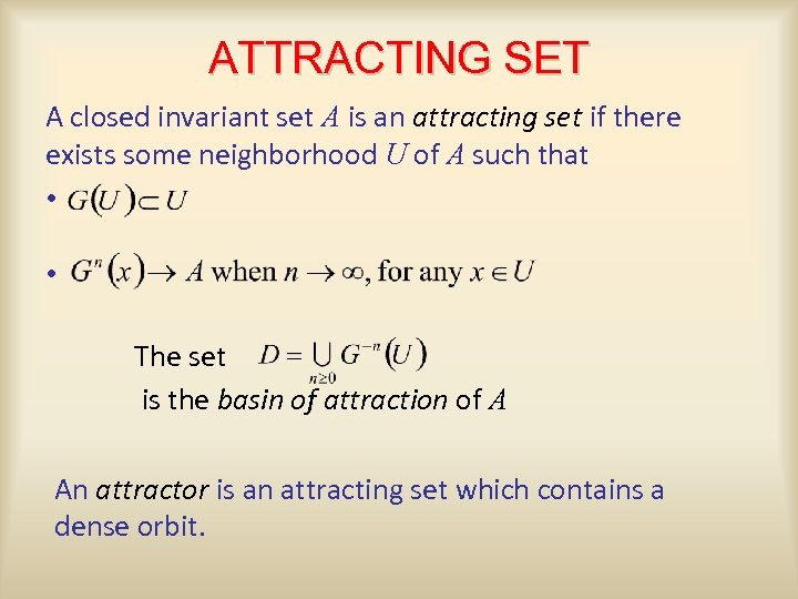ATTRACTING SET A closed invariant set A is an attracting set if there exists some neighborhood U of A such that • • The set is the basin of attraction of A An attractor is an attracting set which contains a dense orbit.

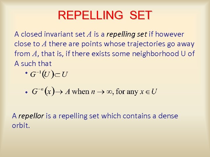REPELLING SET A closed invariant set A is a repelling set if however close to A there are points whose trajectories go away from A, that is, if there exists some neighborhood U of A such that • • A repellor is a repelling set which contains a dense orbit.

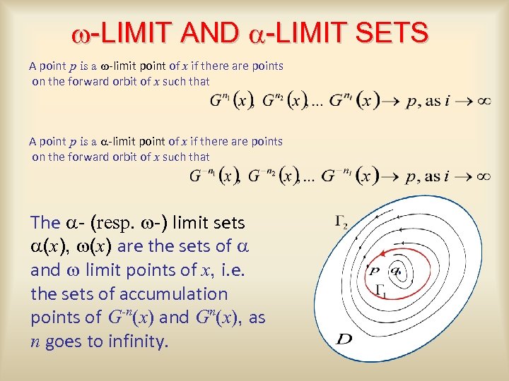w-LIMIT AND a-LIMIT SETS A point p is a w-limit point of x if there are points on the forward orbit of x such that A point p is a a-limit point of x if there are points on the forward orbit of x such that The a- (resp. w-) limit sets a(x), w(x) are the sets of a and w limit points of x, i. e. the sets of accumulation points of G-n(x) and Gn(x), as n goes to infinity.

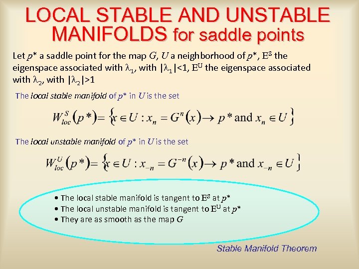LOCAL STABLE AND UNSTABLE MANIFOLDS for saddle points Let p* a saddle point for the map G, U a neighborhood of p*, ES the eigenspace associated with l 1, with |l 1|<1, EU the eigenspace associated with l 2, with |l 2|>1 The local stable manifold of p* in U is the set The local unstable manifold of p* in U is the set • The local stable manifold is tangent to ES at p* • The local unstable manifold is tangent to EU at p* • They are as smooth as the map G Stable Manifold Theorem

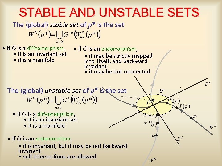STABLE AND UNSTABLE SETS The (global) stable set of p* is the set • If G is a diffeomorphism, • it is an invariant set • it is a manifold • If G is an endomorphism, • it may be strictly mapped into itself, and backward invariant • it may be not connected The (global) unstable set of p* is the set • If G is a diffeomorphism, • it is an invariant set • it is a manifold • If G is an endomorphism, • it is invariant, but it may be not backward invariant • self intersections are allowed U

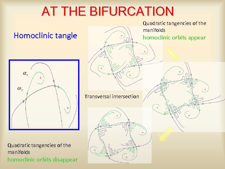
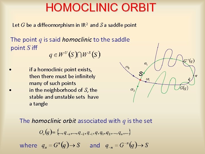HOMOCLINIC ORBIT Let G be a diffeomorphism in IR 2 and S a saddle point The point q is said homoclinic to the saddle point S iff • • if a homoclinic point exists, then there must be infinitely many of such points in the neighborhood of S, the stable and unstable sets have a tangle s The homoclinic orbit associated with q is the set where and

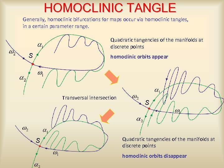HOMOCLINIC TANGLE Generally, homoclinic bifurcations for maps occur via homoclinic tangles, in a certain parameter range. Quadratic tangencies of the manifolds at discrete points S homoclinic orbits appear Transversal intersection S S Quadratic tangencies of the manifolds at discrete points homoclinic orbits disappear

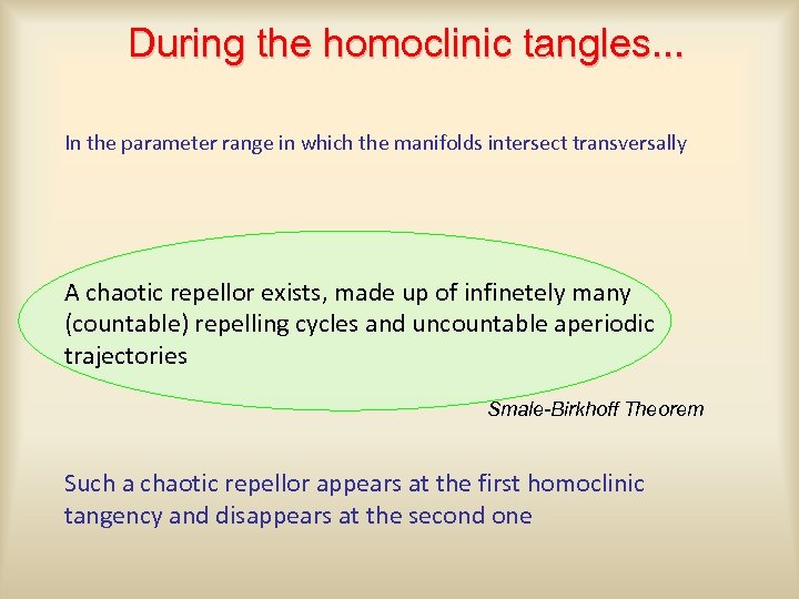During the homoclinic tangles. . . In the parameter range in which the manifolds intersect transversally A chaotic repellor exists, made up of infinetely many (countable) repelling cycles and uncountable aperiodic trajectories Smale-Birkhoff Theorem Such a chaotic repellor appears at the first homoclinic tangency and disappears at the second one

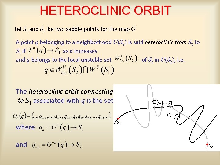HETEROCLINIC ORBIT Let S 1 and S 2 be two saddle points for the map G A point q belonging to a neighborhood U(S 2) is said heteroclinic from S 2 to S 1 if as n increases and q belongs to the local unstable set of S 2 in U(S 2), i. e. The heteroclinic orbit connecting S 2 to S 1 associated with q is the set where and

INVARIANT CLOSED CURVE In a discrete map, a closed curve is an invariant set (i. e. , a set mapped into itself) of the phase-space corresponding to quasi-periodic or periodic trajectories. Neimark-Sacker bifurcation When the eigenvalues of the Jacobian matrix evaluated at the fixed point P* are complex and cross the unit circle then: § with a repelling closed curve GU, existing when P* is still stable subcritical type §

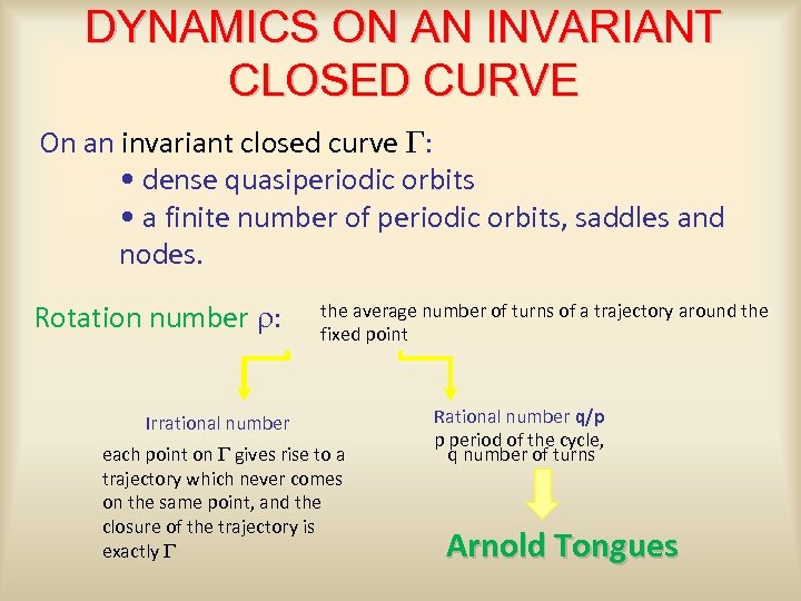DYNAMICS ON AN INVARIANT CLOSED CURVE On an invariant closed curve G: • dense quasiperiodic orbits • a finite number of periodic orbits, saddles and nodes. Rotation number r: the average number of turns of a trajectory around the fixed point Irrational number each point on G gives rise to a trajectory which never comes on the same point, and the closure of the trajectory is exactly G Rational number q/p p period of the cycle, q number of turns Arnold Tongues

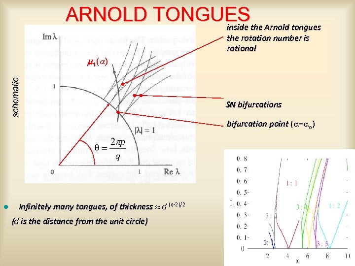ARNOLD TONGUESthe Arnold tongues inside the rotation number is rational schematic m 1 (a ) SN bifurcations bifurcation point (a=ao) l Infinitely many tongues, of thickness d (q-2)/2 (d is the distance from the unit circle) (

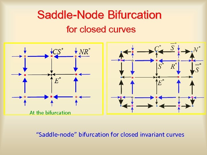
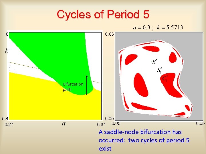
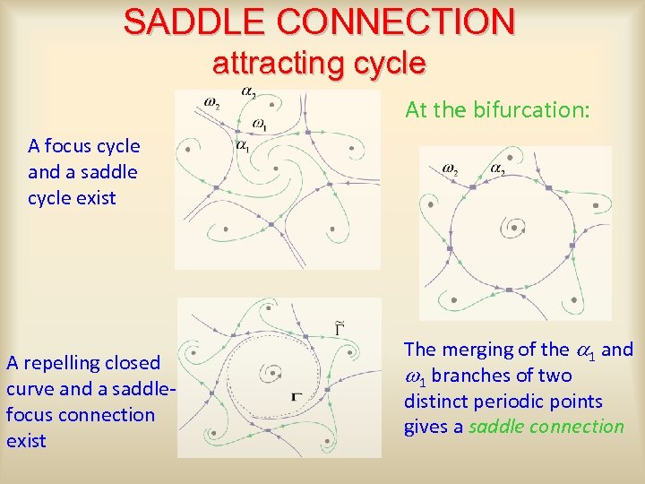
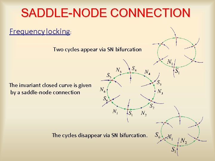SADDLE-NODE CONNECTION Frequency locking: Two cycles appear via SN bifurcation The invariant closed curve is given by a saddle-node connection The cycles disappear via SN bifurcation.

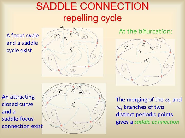
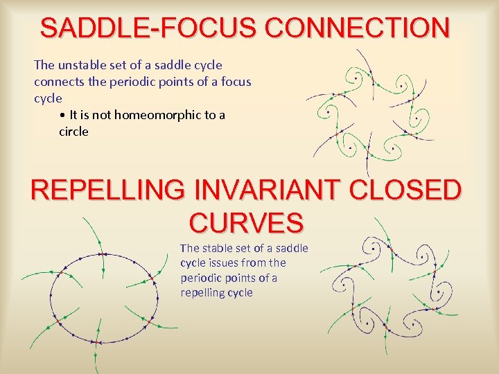SADDLE-FOCUS CONNECTION The unstable set of a saddle cycle connects the periodic points of a focus cycle • It is not homeomorphic to a circle REPELLING INVARIANT CLOSED CURVES The stable set of a saddle cycle issues from the periodic points of a repelling cycle

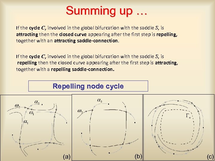
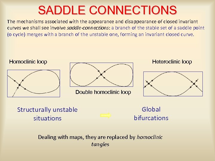SADDLE CONNECTIONS The mechanisms associated with the appearance and disappearance of closed invariant curves we shall see involve saddle-connections: a branch of the stable set of a saddle point (o cycle) merges with a branch of the unstable one, forming an invariant closed curve. Homoclinic loop Heteroclinic loop Double homoclinic loop Structurally unstable situations Global bifurcations Dealing with maps, they are replaced by homoclinic tangles

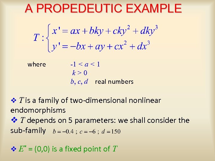A PROPEDEUTIC EXAMPLE where -1 < a < 1 k>0 b, c, d real numbers v T is a family of two-dimensional nonlinear endomorphisms v T depends on 5 parameters: we shall consider the sub-family v E* = (0, 0) is a fixed point of T

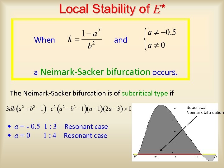Local Stability of E* When and a Neimark-Sacker bifurcation occurs. The Neimark-Sacker bifurcation is of subcritical type if Subcritical Neimark bifurcation • a = - 0. 5 1 : 3 Resonant case • a=0 1 : 4 Resonant case

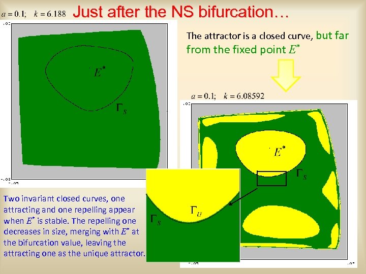Just after the NS bifurcation… The attractor is a closed curve, but far from the fixed point E* Two invariant closed curves, one attracting and one repelling appear when E* is stable. The repelling one decreases in size, merging with E* at the bifurcation value, leaving the attracting one as the unique attractor.

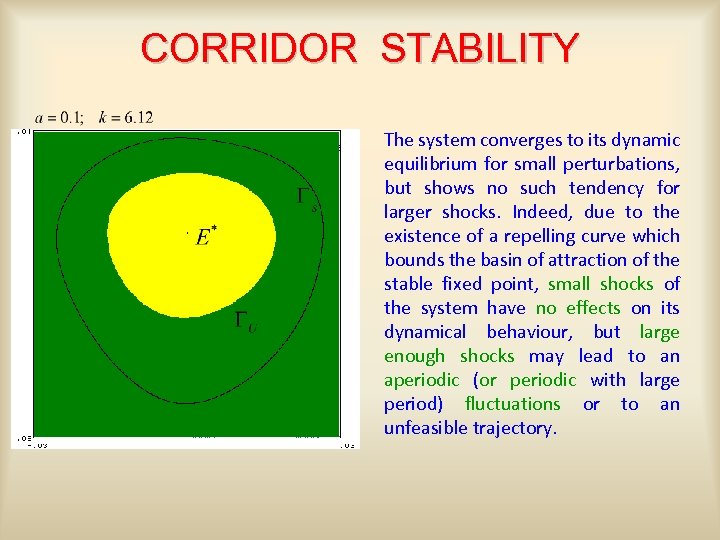CORRIDOR STABILITY The system converges to its dynamic equilibrium for small perturbations, but shows no such tendency for larger shocks. Indeed, due to the existence of a repelling curve which bounds the basin of attraction of the stable fixed point, small shocks of the system have no effects on its dynamical behaviour, but large enough shocks may lead to an aperiodic (or periodic with large period) fluctuations or to an unfeasible trajectory.

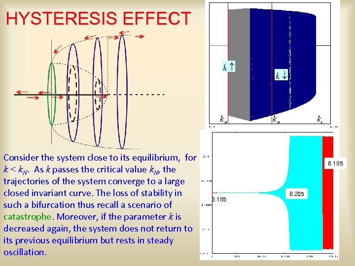HYSTERESIS EFFECT Consider the system close to its equilibrium, for k < k. N. As k passes the critical value k. N, the trajectories of the system converge to a large closed invariant curve. The loss of stability in such a bifurcation thus recall a scenario of catastrophe. Moreover, if the parameter k is decreased again, the system does not return to its previous equilibrium but rests in steady oscillation. 6. 185 6. 205

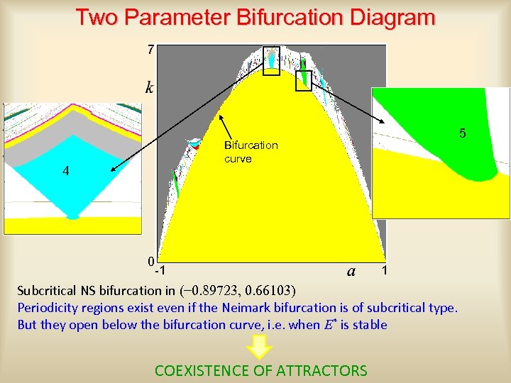Two Parameter Bifurcation Diagram 7 5 Bifurcation curve 4 0 -1 1 Subcritical NS bifurcation in (− 0. 89723, 0. 66103) Periodicity regions exist even if the Neimark bifurcation is of subcritical type. But they open below the bifurcation curve, i. e. when E* is stable COEXISTENCE OF ATTRACTORS

Square Separate Map 0. 015 0. 02 -0. 05 0. 03

Saddle-Node Bifurcation for closed curves At the bifurcation “Saddle-node” bifurcation for closed invariant curves

Cycles of Period 5 0. 03 6 Bifurcation path 5. 4 0. 27 -0. 05 0. 31 -0. 05 A saddle-node bifurcation has occurred: two cycles of period 5 exist 0. 05

0. 015 -0. 02 Appearance of Closed Curves 0. 03

Enlargement in

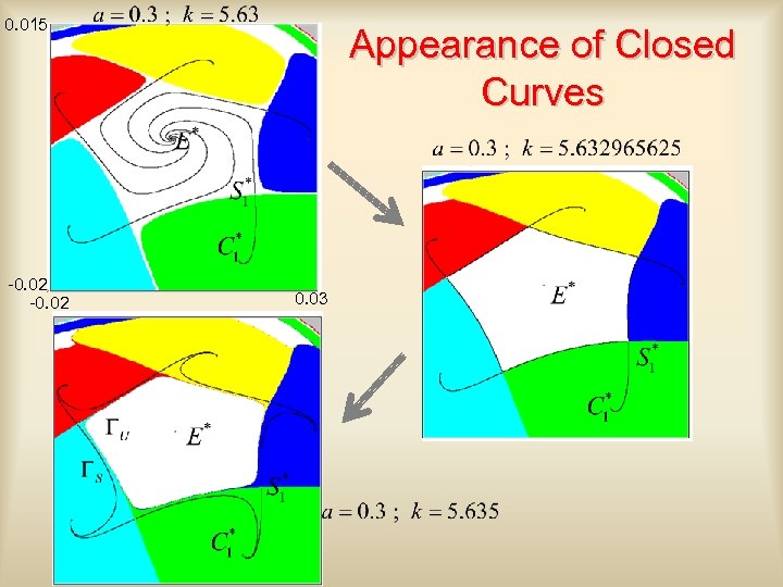
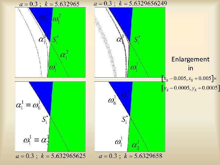
SADDLE CONNECTION attracting cycle At the bifurcation: A focus cycle and a saddle cycle exist A repelling closed curve and a saddlefocus connection exist The merging of the a 1 and w 1 branches of two distinct periodic points gives a saddle connection

SADDLE CONNECTION repelling cycle A focus cycle and a saddle cycle exist An attracting closed curve and a saddle-focus connection exist At the bifurcation: The merging of the a 1 and w 1 branches of two distinct periodic points gives a saddle connection

Summing up … If the cycle C, involved in the global bifurcation with the saddle S, is attracting then the closed curve appearing after the first step is repelling, together with an attracting saddle-connection. If the cycle C, involved in the global bifurcation with the saddle S, is repelling then the closed curve appearing after the first step is attracting, together with a repelling saddle-connection. Repelling node cycle (a) (b) (c)

AT THE BIFURCATION Quadratic tangencies of the manifolds Homoclinic tangle homoclinic orbits appear Transversal intersection Quadratic tangencies of the manifolds homoclinic orbits disappear

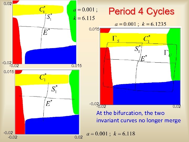0. 02 Period 4 Cycles 0. 015 -0. 02 At the bifurcation, the two invariant curves no longer merge -0. 02

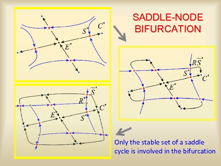SADDLE-NODE BIFURCATION Only the stable set of a saddle cycle is involved in the bifurcation

A financial market with imitators The model describes a single asset stock market where n is the number of traders (i=1, . . . , n) is the investment attitude of agent i s. t. if agent i wants to buy an asset’s unit at t (optimistic investor) if agent i wants to sell an asset’s unit at t (pessimistic investor) The investors’ average opinion is, then, Let nb and ns be the totality of buyers and sellers with nb + ns= n Thus, we get

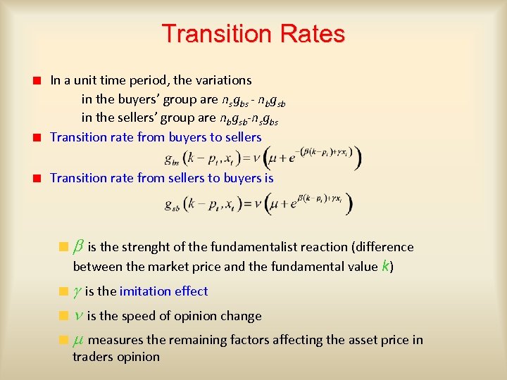Transition Rates In a unit time period, the variations in the buyers’ group are nsgbs - nbgsb in the sellers’ group are nbgsb-nsgbs Transition rate from buyers to sellers Transition rate from sellers to buyers is b is the strenght of the fundamentalist reaction (difference between the market price and the fundamental value k) g is the imitation effect n is the speed of opinion change m measures the remaining factors affecting the asset price in traders opinion

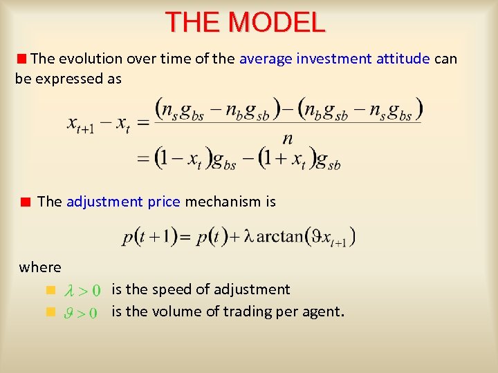THE MODEL The evolution over time of the average investment attitude can be expressed as The adjustment price mechanism is where is the speed of adjustment is the volume of trading per agent.

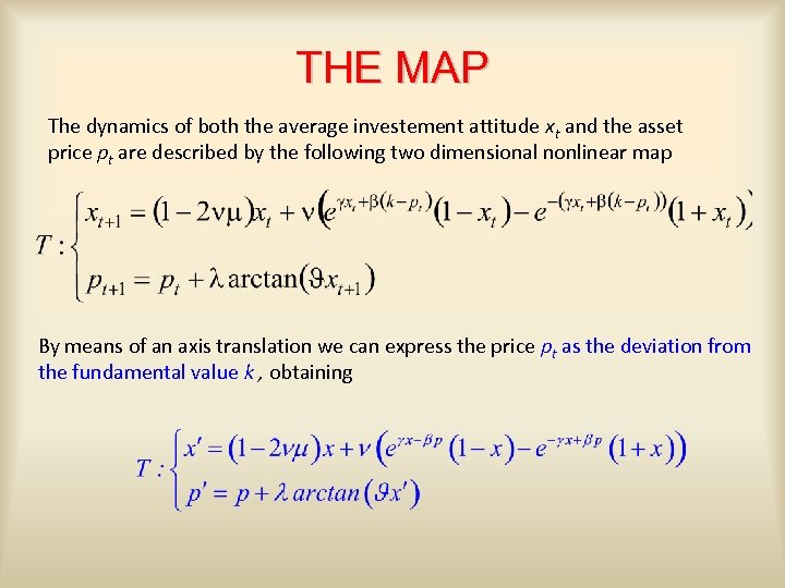THE MAP The dynamics of both the average investement attitude xt and the asset price pt are described by the following two dimensional nonlinear map By means of an axis translation we can express the price pt as the deviation from the fundamental value k , obtaining

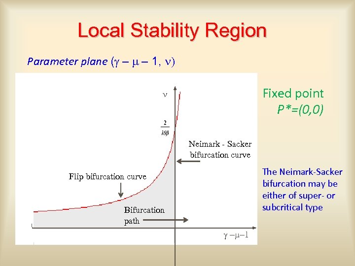Local Stability Region Parameter plane (g – m – 1, n) Fixed point P*=(0, 0) n Neimark - Sacker bifurcation curve The Neimark-Sacker bifurcation may be either of super- or subcritical type Flip bifurcation curve Bifurcation path g -m-1

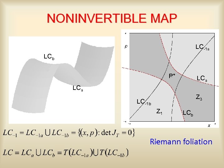NONINVERTIBLE MAP p LC-1 a LCb P* LCa Z 3 LC-1 b Z 1 LCb x Riemann foliation

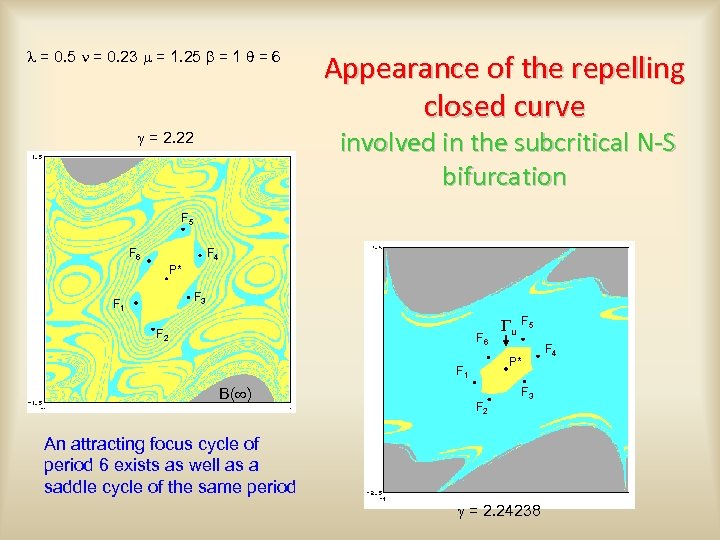l = 0. 5 n = 0. 23 m = 1. 25 b = 1 q = 6 Appearance of the repelling closed curve involved in the subcritical N-S bifurcation g = 2. 22 F 5 F 4 F 6 P* F 3 F 1 F 2 F 6 P* F 1 B( ) Gu F 5 F 3 F 2 An attracting focus cycle of period 6 exists as well as a saddle cycle of the same period g = 2. 24238 F 4

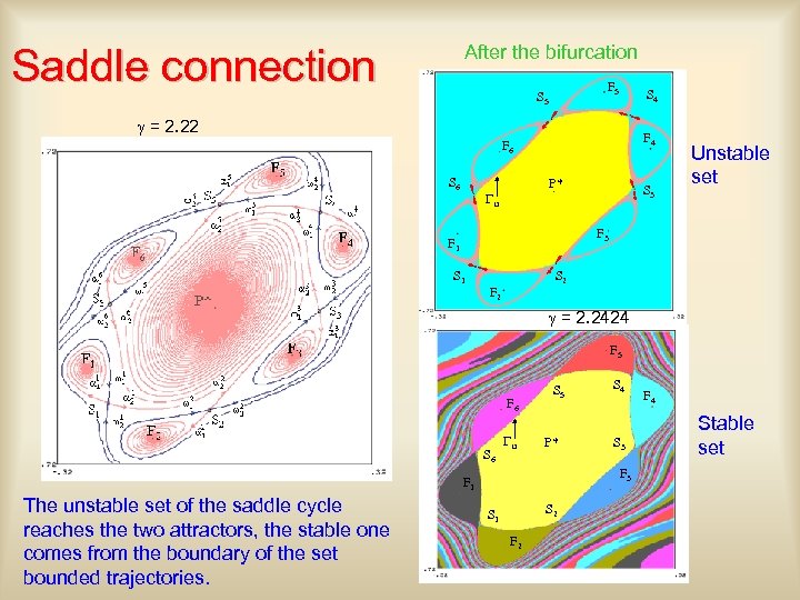Saddle connection After the bifurcation F 5 S 4 g = 2. 22 F 4 F 6 S 6 P* Gu S 3 Unstable set F 3 F 1 S 2 F 2 g = 2. 2424 F 5 F 6 S 6 Gu S 5 P* S 3 F 1 The unstable set of the saddle cycle reaches the two attractors, the stable one comes from the boundary of the set bounded trajectories. S 4 S 2 S 1 F 2 F 4 Stable set

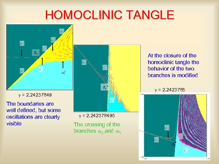HOMOCLINIC TANGLE S 1 At the closure of the homoclinic tangle the behavior of the two branches is modified S 1 g = 2. 24237849 The boundaries are well defined, but some oscillations are clearly visible g = 2. 2423785 g = 2. 242378495 The crossing of the branches a 2 and w 1 S 1

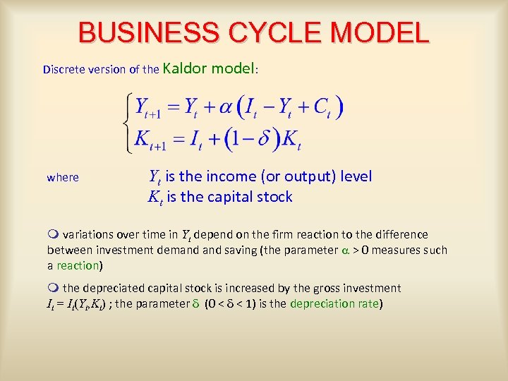BUSINESS CYCLE MODEL Discrete version of the Kaldor where model: Yt is the income (or output) level Kt is the capital stock m variations over time in Yt depend on the firm reaction to the difference between investment demand saving (the parameter a > 0 measures such a reaction) m the depreciated capital stock is increased by the gross investment It = It(Yt, Kt) ; the parameter d (0 < d < 1) is the depreciation rate)

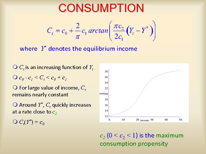CONSUMPTION where Y* denotes the equilibrium income m Ct is an increasing function of Yt m c 0 - c 1 < C t < c 0 + c 1 m For large value of income, Ct remains nearly constant m Around Y*, Ct quickly increases at a rate close to c 2 m Ct(Y*) = c 0 c 2 (0 < c 2 < 1) is the maximum consumption propensity

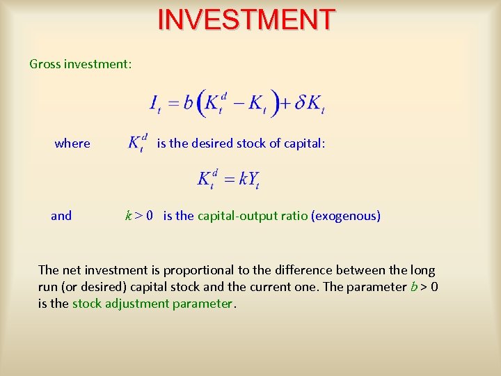INVESTMENT Gross investment: where and is the desired stock of capital: k > 0 is the capital-output ratio (exogenous) The net investment is proportional to the difference between the long run (or desired) capital stock and the current one. The parameter b > 0 is the stock adjustment parameter.

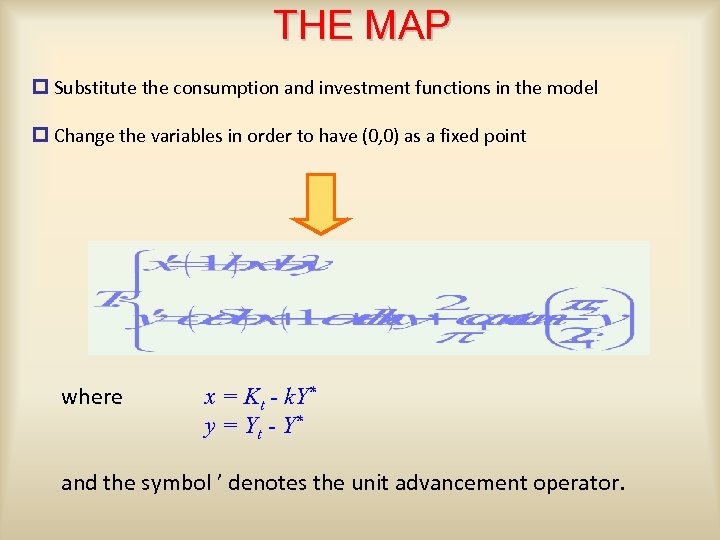THE MAP p Substitute the consumption and investment functions in the model p Change the variables in order to have (0, 0) as a fixed point where x = Kt - k. Y* y = Y t - Y* and the symbol ’ denotes the unit advancement operator.

PROPERTIES OF T m It depends on 6 parameters: a, d, k, b, c 1, c 2 : in our analysis m It is symmetric with respect to the origin m It is invertible if holds. Otherwise it is a Z 1 -Z 3 -Z 1 map. In our analysis we shall consider a parameter range in which T is invertible.

FIXED POINTS m If the map T has a unique fixed point m If two further fixed points exist, P* and Q*, symmetric with respect to E* They are such that x = ky and y can be obtained from the equation

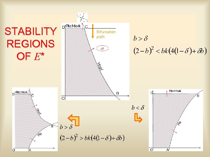STABILITY REGIONS OF E* Bifurcation path

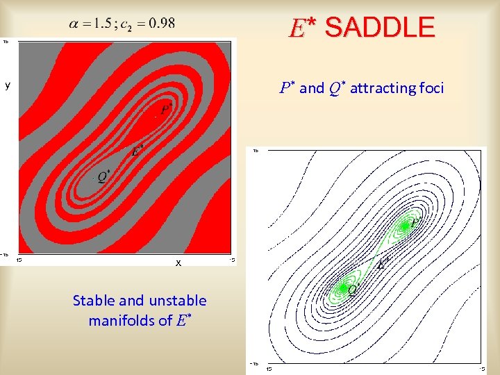E* SADDLE P* and Q* attracting foci y x Stable and unstable manifolds of E*

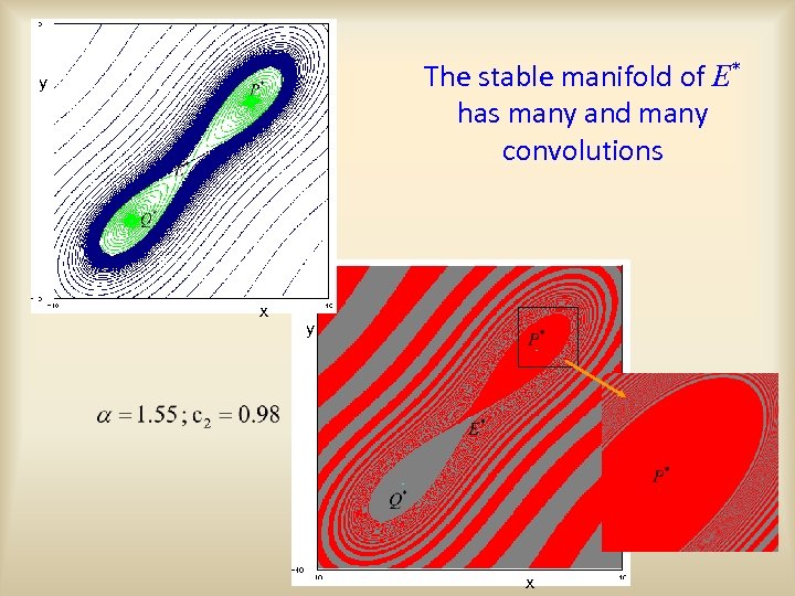The stable manifold of E* has many and many convolutions y x

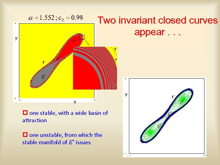Two invariant closed curves appear. . . y y x p one stable, with a wide basin of attraction p one unstable, from which the stable manifold of E* issues

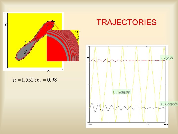TRAJECTORIES y x x t

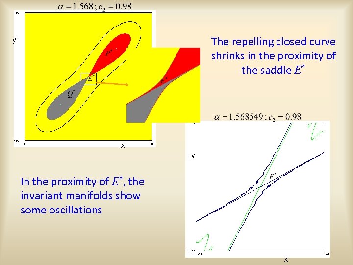The repelling closed curve shrinks in the proximity of the saddle E* y x y In the proximity of E*, the invariant manifolds show some oscillations x

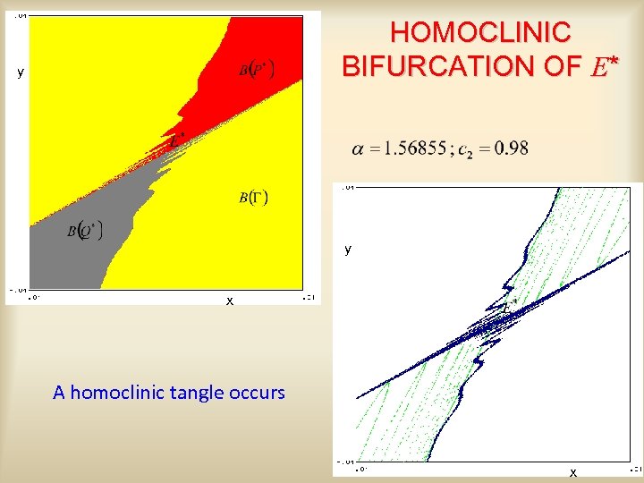HOMOCLINIC BIFURCATION OF E* y y x A homoclinic tangle occurs x

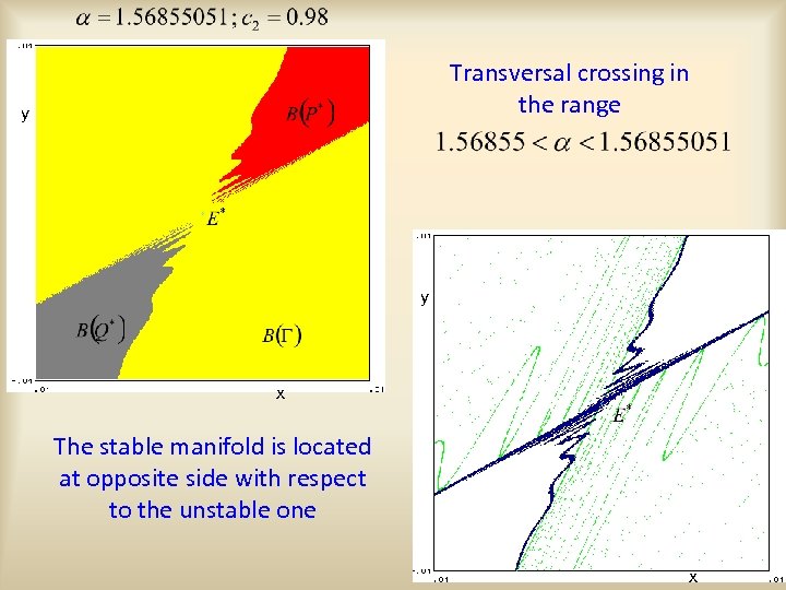Transversal crossing in the range y y x The stable manifold is located at opposite side with respect to the unstable one x

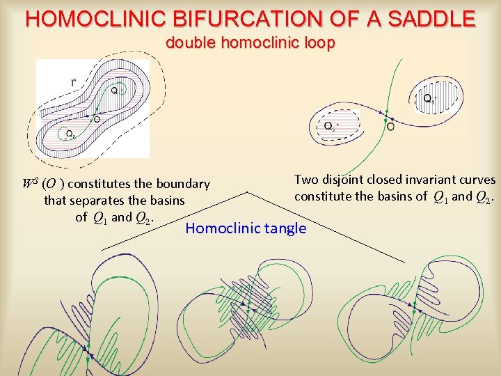HOMOCLINIC BIFURCATION OF A SADDLE double homoclinic loop WS (O ) constitutes the boundary that separates the basins of Q 1 and Q 2. Two disjoint closed invariant curves constitute the basins of Q 1 and Q 2. Homoclinic tangle

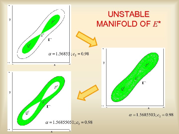UNSTABLE MANIFOLD OF E* y x y y x x

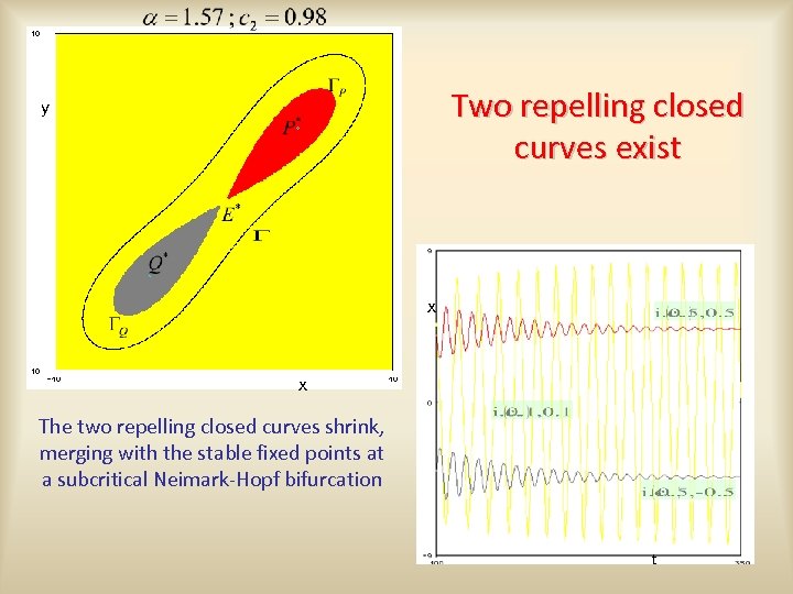Two repelling closed curves exist y x x The two repelling closed curves shrink, merging with the stable fixed points at a subcritical Neimark-Hopf bifurcation t

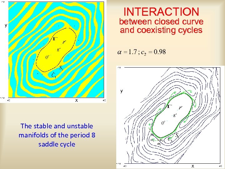INTERACTION between closed curve and coexisting cycles y y x The stable and unstable manifolds of the period 8 saddle cycle x

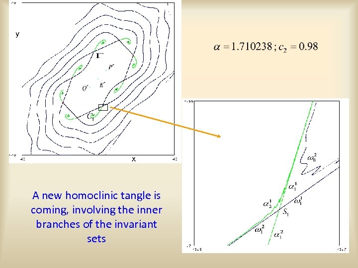y x A new homoclinic tangle is coming, involving the inner branches of the invariant sets

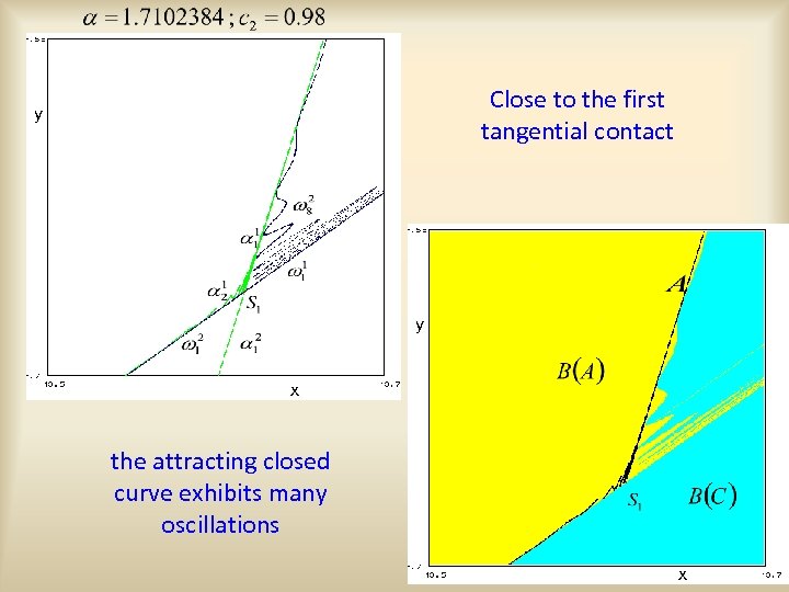Close to the first tangential contact y y x the attracting closed curve exhibits many oscillations x

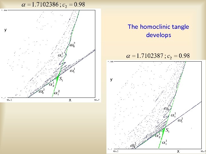The homoclinic tangle develops y y x x

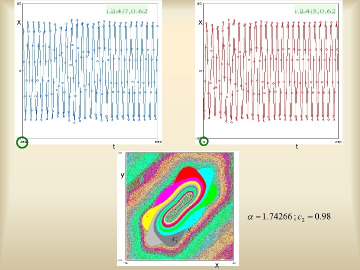
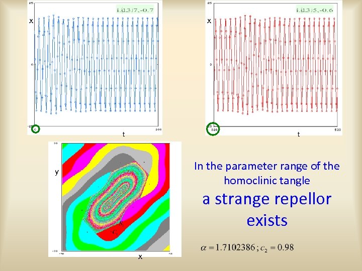x x t t In the parameter range of the homoclinic tangle y a strange repellor exists x

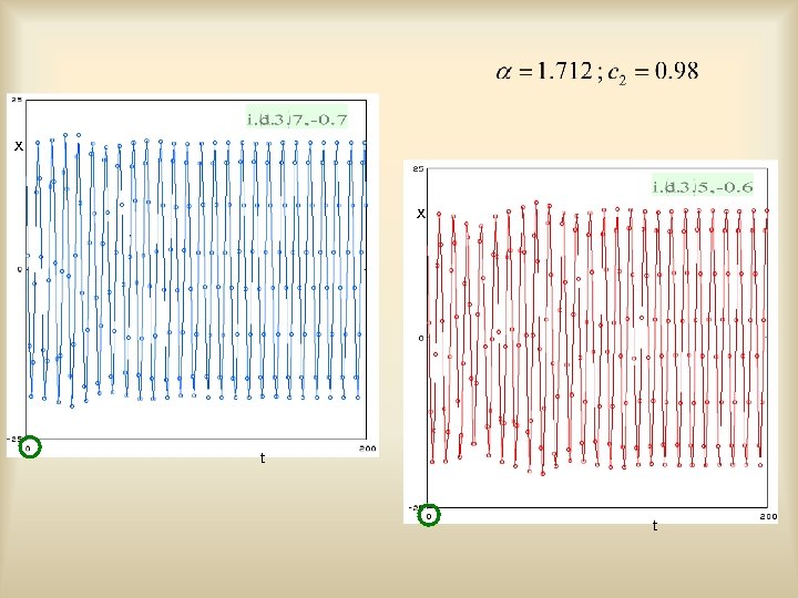x x t t

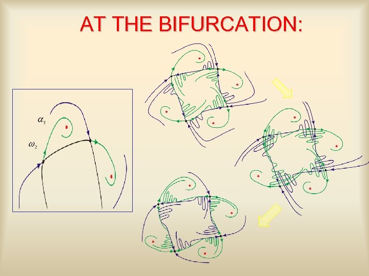
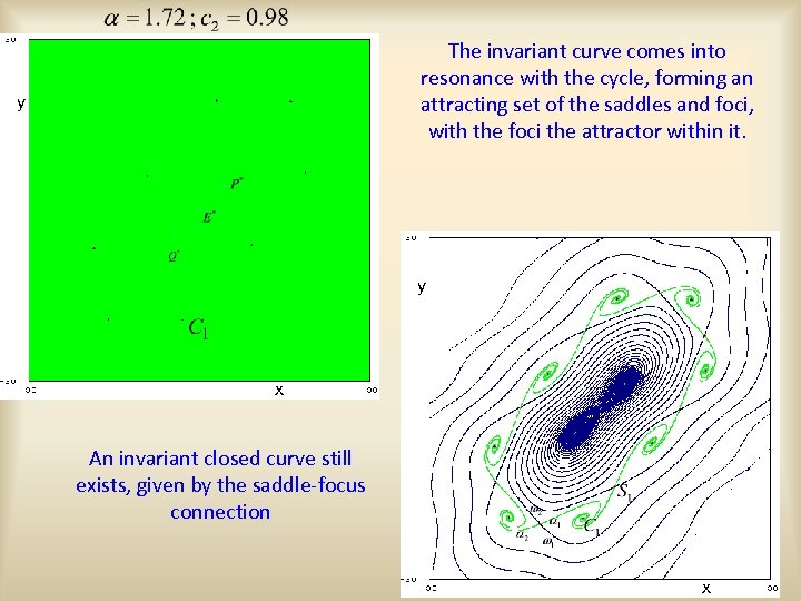
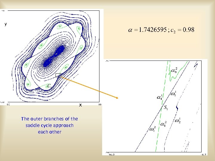
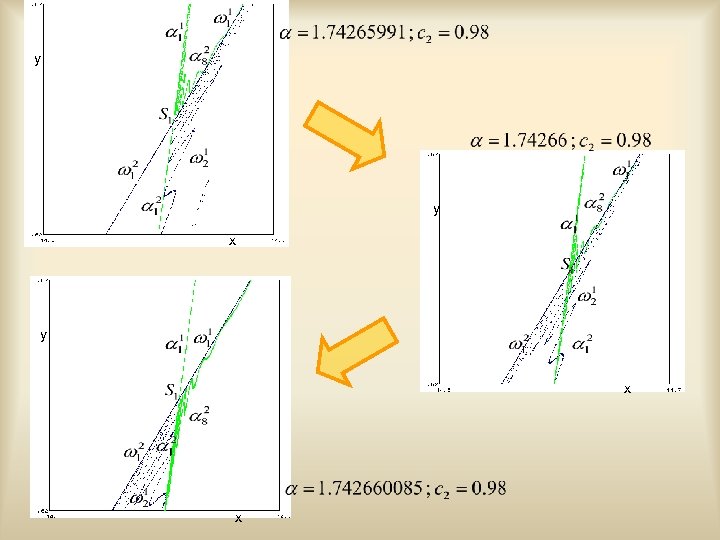
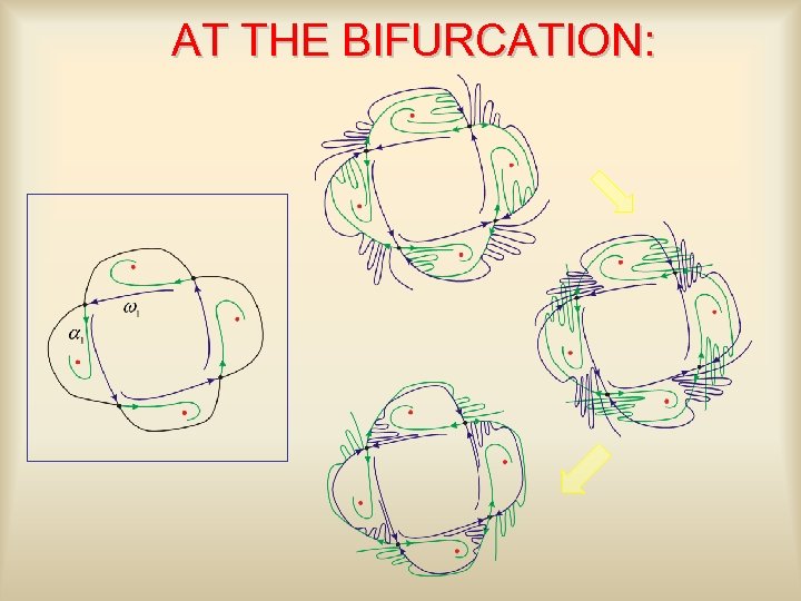
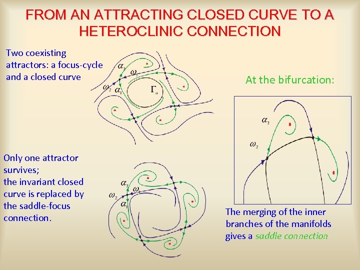FROM AN ATTRACTING CLOSED CURVE TO A HETEROCLINIC CONNECTION Two coexisting attractors: a focus-cycle and a closed curve Only one attractor survives; the invariant closed curve is replaced by the saddle-focus connection. At the bifurcation: The merging of the inner branches of the manifolds gives a saddle connection

AT THE BIFURCATION:

The invariant curve comes into resonance with the cycle, forming an attracting set of the saddles and foci, with the foci the attractor within it. y y x An invariant closed curve still exists, given by the saddle-focus connection x

y x The outer branches of the saddle cycle approach each other

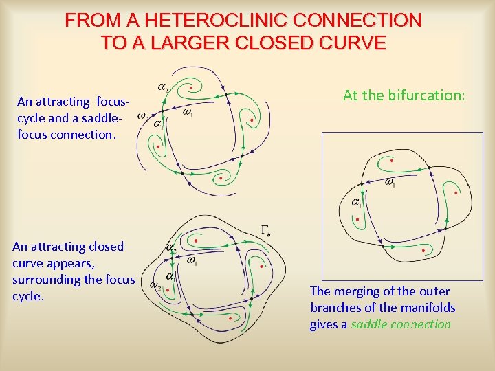FROM A HETEROCLINIC CONNECTION TO A LARGER CLOSED CURVE An attracting focuscycle and a saddlefocus connection. An attracting closed curve appears, surrounding the focus cycle. At the bifurcation: The merging of the outer branches of the manifolds gives a saddle connection

y y x x

AT THE BIFURCATION:

x x t t y x

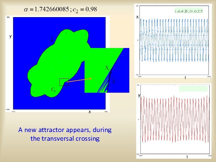x y t y x A new attractor appears, during the transversal crossing t

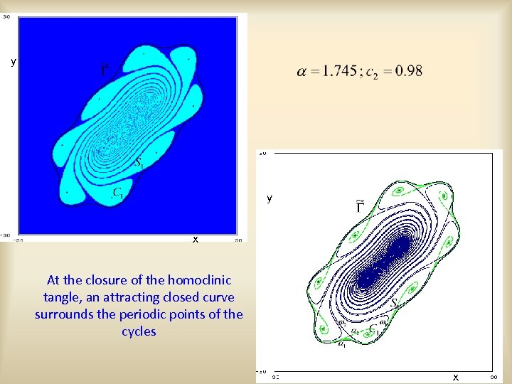y y x At the closure of the homoclinic tangle, an attracting closed curve surrounds the periodic points of the cycles x

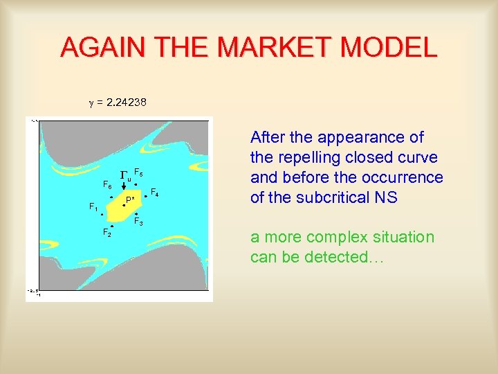AGAIN THE MARKET MODEL g = 2. 24238 F 6 Gu F 5 P* F 1 F 4 After the appearance of the repelling closed curve and before the occurrence of the subcritical NS F 3 F 2 a more complex situation can be detected…

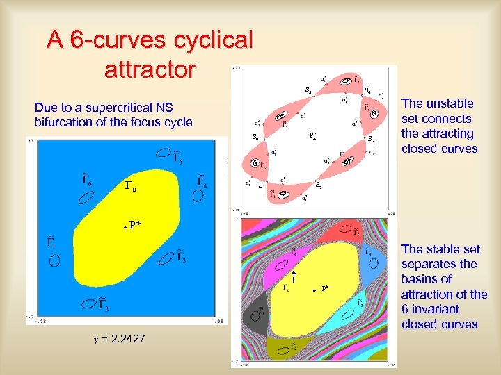A 6 -curves cyclical attractor S 5 S 4 Due to a supercritical NS bifurcation of the focus cycle P* S 6 Gu S 1 S 3 The unstable set connects the attracting closed curves S 2 P* P* g = 2. 2427 The stable set separates the basins of attraction of the 6 invariant closed curves

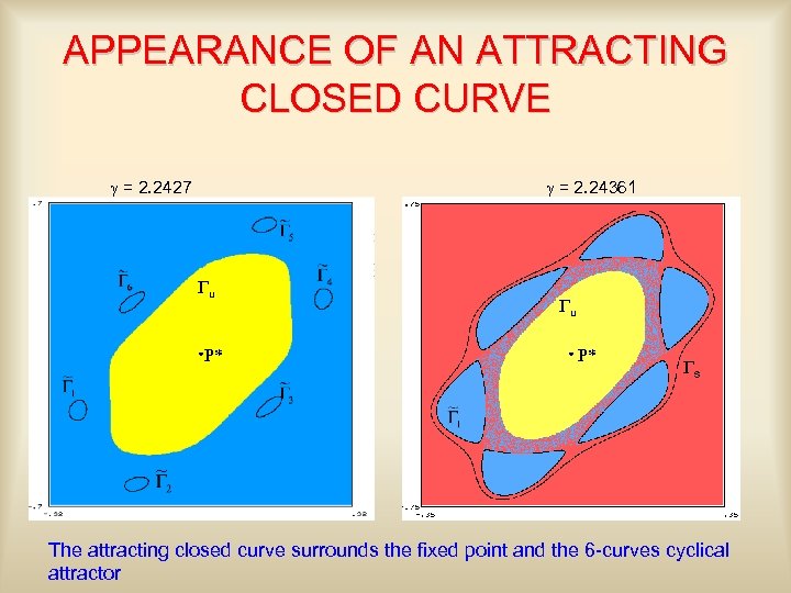APPEARANCE OF AN ATTRACTING CLOSED CURVE g = 2. 2427 g = 2. 24361 Gu P* Gs The attracting closed curve surrounds the fixed point and the 6 -curves cyclical attractor

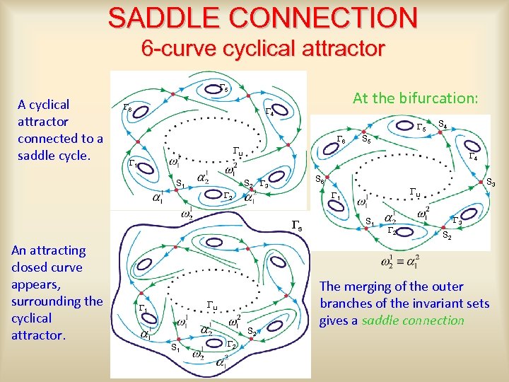SADDLE CONNECTION 6 -curve cyclical attractor G 5 A cyclical attractor connected to a saddle cycle. G 6 At the bifurcation: G 4 G 5 G 6 Gu G 1 S 6 Gs Gu G 1 S 2 S 1 G 2 S 3 Gu G 1 G 2 An attracting closed curve appears, surrounding the cyclical attractor. S 5 G 4 S 2 G 3 S 1 S 4 S 1 G 2 G 3 S 2 The merging of the outer branches of the invariant sets gives a saddle connection

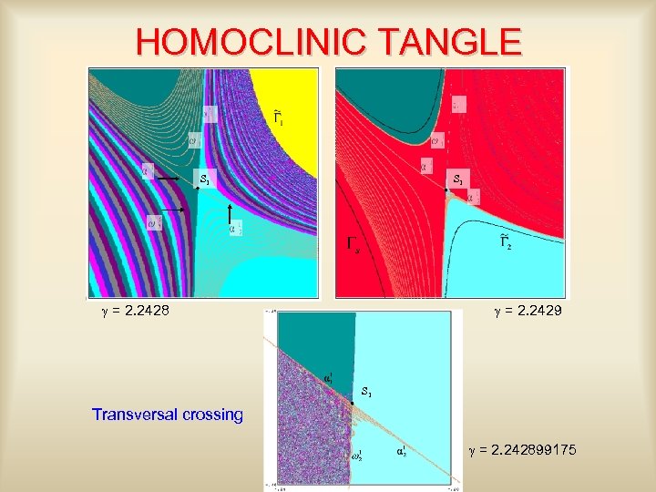HOMOCLINIC TANGLE S 1 g = 2. 2428 g = 2. 2429 S 1 Transversal crossing g = 2. 242899175

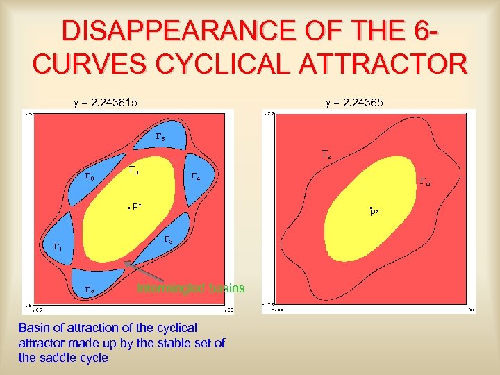DISAPPEARANCE OF THE 6 CURVES CYCLICAL ATTRACTOR g = 2. 243615 g = 2. 24365 G 5 Gs G 6 Gu G 4 P* P* G 3 G 1 G 2 Gu Intermingled basins Basin of attraction of the cyclical attractor made up by the stable set of the saddle cycle

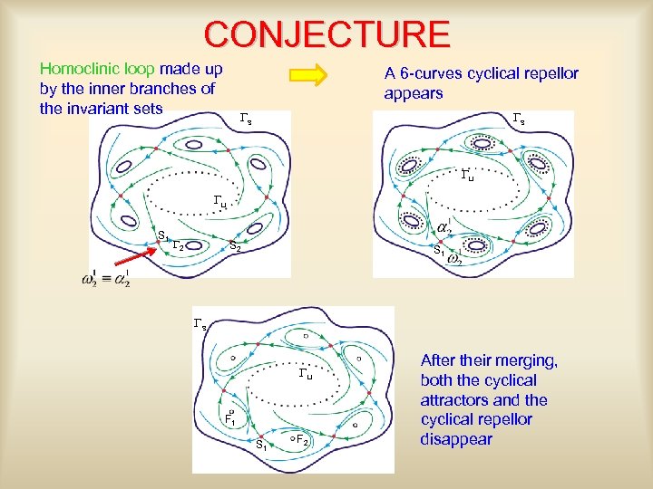CONJECTURE Homoclinic loop made up by the inner branches of the invariant sets A 6 -curves cyclical repellor appears Gs Gs Gu Gu S 1 G 2 S 1 Gs Gu F 1 S 1 F 2 After their merging, both the cyclical attractors and the cyclical repellor disappear

MAIN REFERENCES Global bifurcations of invariant closed curves - AA, G. I. Bischi, R. Dieci, L. Gardini (2005) "Global bifurcations of closed invariant curves in twodimensional maps: A computer assisted study" International Journal of Bifurcations and Chaos, vol. 15 (4), pp. 1285 -1328 -AA, G. I. Bischi, R. Dieci, L. Gardini (2006) "Homoclinic tangles associated with closed invariant curves in families of 2 D maps" Grazer Math. Ber. N. 350, pp. 1 -14 Appearance/disappearance of invariant closed curves - AA (2007), On the bifurcation mechanisms causing the appearance of invariant closed curves, Grazer Math. Ber. , N. 351, pp. 1 -20 - AA, Gardini, Puu (2005), Some global bifurcations related to the appearance of closed invariant curves, Computers and Mathematics in Simulation 68, pp. 201 -219 -AA (2006) Homoclinic connections and subcritical Neimark bifurcations in a duopoly model with adaptively adjusted productions, Chaos Solitons & Fractals 29, pp. 739 -755 - I. Foroni, AA (2010) “Complex dynamics associated with the appearance/disappearance of invariant closed curves” Submitted Interactions between coexisting closed curves and cycles - AA, Dieci R. (2006), Coexistence of attractors and homoclinic loops in a Kaldor-like business cycle model, In: T. Puu and I Sushko (eds. ): Business cycle dynamics: Models and tools. Springer-Verlag, pp. 223 -254 -AA, Dieci R. , Gardini L. (2007), Homoclinic tangle in Kaldor's like business cycle models, Journal of Economic Behavior and Organization 62, pp. 324 -347 … and references therein