TUTORIAL Randomized Algorithms for Matrices and Massive Data

Скачать презентацию TUTORIAL Randomized Algorithms for Matrices and Massive Data

4543a05a51811bb51fe1b67942a6a593.ppt

Количество слайдов: 152

TUTORIAL: Randomized Algorithms for Matrices and Massive Data Sets Petros Drineas Michael W. Mahoney RPI Dept. of Computer Science Yale University Dept. of Mathematics (now at Yahoo! Research) (Most recent copy) available at: http: //www. cs. yale. edu/homes/mmahoney http: //www. cs. rpi. edu/~drinep

Randomized Linear Algebra Algorithms Goal: To develop and analyze (fast) Monte Carlo algorithms for performing useful computations on large matrices and tensors. • Matrix Multiplication • Computation of the Singular Value Decomposition • Computation of the CUR Decomposition • Testing Feasibility of Linear Programs • Least Squares Approximation • Tensor computations: SVD generalizations • Tensor computations: CUR generalization Such computations generally require time which is superlinear in the number of nonzero elements of the matrix/tensor, e. g. , O(n 3) for n £ n matrices. 2

Randomized Linear Algebra Algorithms Motivation: • (Algorithmic) To speed up computations in applications where extremely large data sets are modeled by matrices/tensors and, e. g. , O(n 3) time is not an option. • (Algorithmic) To reduce the memory requirements in applications where the data sets are modeled by matrices/tensors, and storing the whole data is not an option, because the data sets are extremely large. • (Equivalent to the above) To provide some analysis of the performance of the accuracy performance of simple algorithms when only a small sample of the full data set is available. • (Structural) To reveal novel structural properties of the datasets, given sufficient computational time. 3

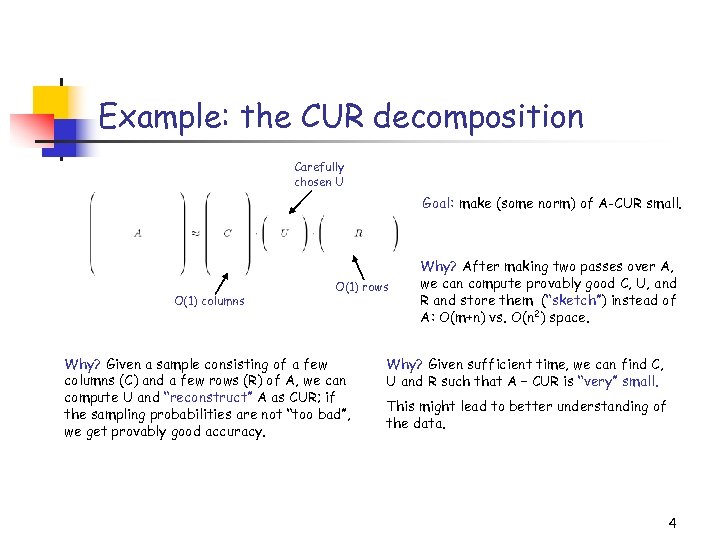Example: the CUR decomposition Carefully chosen U Goal: make (some norm) of A-CUR small. O(1) columns O(1) rows Why? Given a sample consisting of a few columns (C) and a few rows (R) of A, we can compute U and “reconstruct” A as CUR; if the sampling probabilities are not “too bad”, we get provably good accuracy. Why? After making two passes over A, we can compute provably good C, U, and R and store them (“sketch”) instead of A: O(m+n) vs. O(n 2) space. Why? Given sufficient time, we can find C, U and R such that A – CUR is “very” small. This might lead to better understanding of the data. 4

Applications of such algorithms Matrices arise, e. g. , since m objects (documents, genomes, images, web pages), each with n features, may be represented by an m x n matrix A. • Covariance Matrices • Latent Semantic Indexing • DNA Microarray Data • Eigenfaces and Image Recognition • Similarity Queries • Matrix Reconstruction • LOTS of other data applications!! More generally, • Linear and Nonlinear Programming Applications • Design of Approximation Algorithms • Statistical Learning Theory Applications 5

Overview (1/3) • Data Streaming Models and Random Sampling • Matrix Multiplication • Feasibility testing of Linear Programs • Singular Value Decomposition • Sampling rows/columns to approximate singular vectors/values • Sampling elements to approximate singular vectors/values • CUR Matrix Decomposition • Lower bounds on sampling complexities 6

Overview (2/3) • Applications of Matrix CUR • Designing approximation algorithms • Data mining • Microarray data • Recommendation Systems • Tensor-based data sets • Tensor-CUR • Applications of Tensor-CUR • Hyperspectral data • Recommendation systems 7

Overview (3/3) • Kernel-CUR and the Nystrom Method • Regression problems • Least squares problems • The CUR algorithm revisited • A general bound • Iterative sampling of rows/columns • “Optimal” choices of rows/columns • Application: finding ht-SNPs • Conclusions & open problems 8

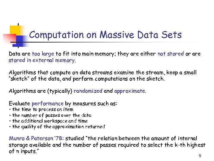Computation on Massive Data Sets Data are too large to fit into main memory; they are either not stored or are stored in external memory. Algorithms that compute on data streams examine the stream, keep a small “sketch” of the data, and perform computations on the sketch. Algorithms are (typically) randomized and approximate. Evaluate performance by measures such as: • the time to process an item • the number of passes over the data • the additional workspace and time • the quality of the approximation returned Munro & Paterson ’ 78: studied “the relation between the amount of internal storage available and the number of passes required to select the k-th highest of n inputs. ” 9

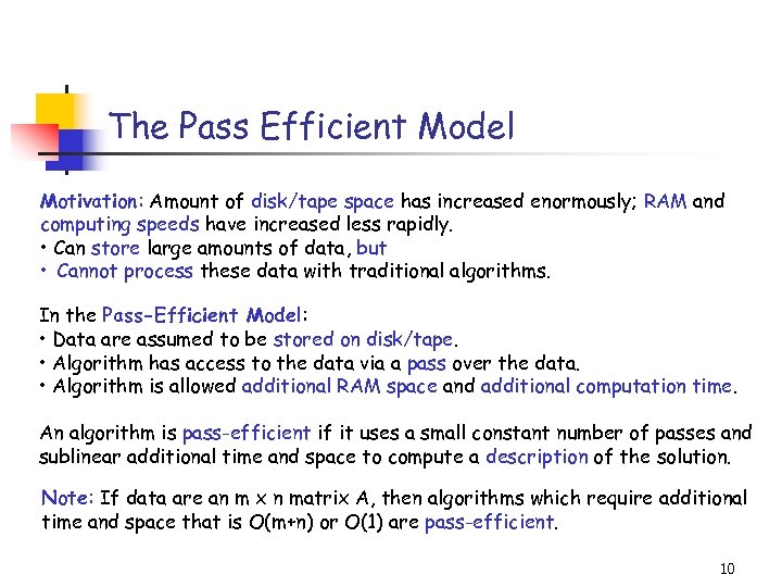The Pass Efficient Model Motivation: Amount of disk/tape space has increased enormously; RAM and computing speeds have increased less rapidly. • Can store large amounts of data, but • Cannot process these data with traditional algorithms. In the Pass-Efficient Model: • Data are assumed to be stored on disk/tape. • Algorithm has access to the data via a pass over the data. • Algorithm is allowed additional RAM space and additional computation time. An algorithm is pass-efficient if it uses a small constant number of passes and sublinear additional time and space to compute a description of the solution. Note: If data are an m x n matrix A, then algorithms which require additional time and space that is O(m+n) or O(1) are pass-efficient. 10

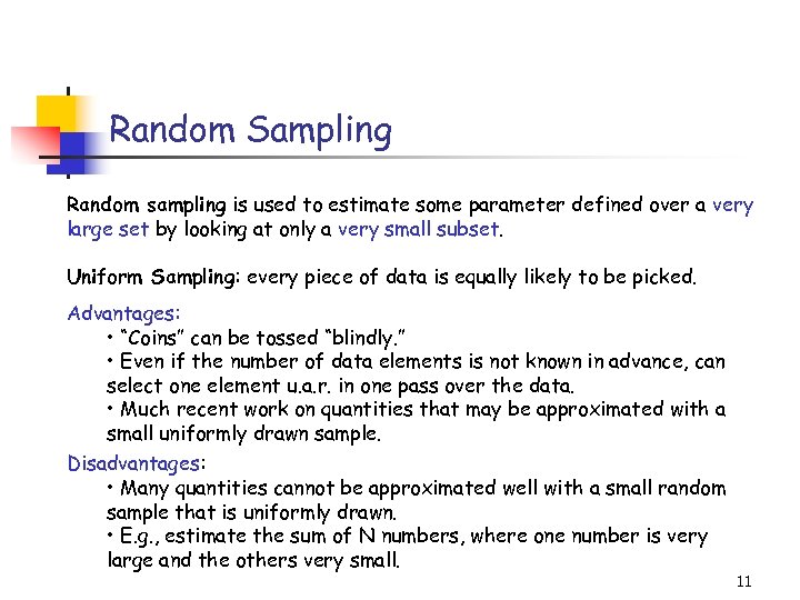Random Sampling Random sampling is used to estimate some parameter defined over a very large set by looking at only a very small subset. Uniform Sampling: every piece of data is equally likely to be picked. Advantages: • “Coins” can be tossed “blindly. ” • Even if the number of data elements is not known in advance, can select one element u. a. r. in one pass over the data. • Much recent work on quantities that may be approximated with a small uniformly drawn sample. Disadvantages: • Many quantities cannot be approximated well with a small random sample that is uniformly drawn. • E. g. , estimate the sum of N numbers, where one number is very large and the others very small. 11

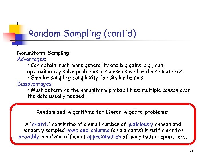Random Sampling (cont’d) Nonuniform Sampling: Advantages: • Can obtain much more generality and big gains, e. g. , can approximately solve problems in sparse as well as dense matrices. • Smaller sampling complexity for similar bounds. Disadvantages: • Must determine the nonuniform probabilities; multiple passes over the data usually needed. Randomized Algorithms for Linear Algebra problems: A “sketch” consisting of a small number of judiciously chosen and randomly sampled rows and columns (or elements) is sufficient for provably rapid and efficient approximation of many matrix operations. 12

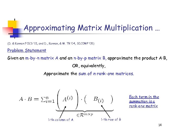Approximating Matrix Multiplication … (D. & Kannan FOCS ’ 01, and D. , Kannan, & M. TR ’ 04, SICOMP ’ 05) Problem Statement Given an m-by-n matrix A and an n-by-p matrix B, approximate the product A·B, OR, equivalently, Approximate the sum of n rank-one matrices. Each term in the summation is a rank-one matrix i-th column of A i-th row of B 14

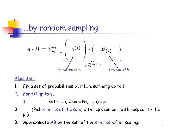…by random sampling i-th column of A i-th row of B Algorithm 1. Fix a set of probabilities pi, i=1…n, summing up to 1. 2. For t=1 up to s, 1. 3. 3. pi. ) set jt = i, where Pr(jt = i) = pi; (Pick s terms of the sum, with replacement, with respect to the Approximate AB by the sum of the s terms, after scaling. 15

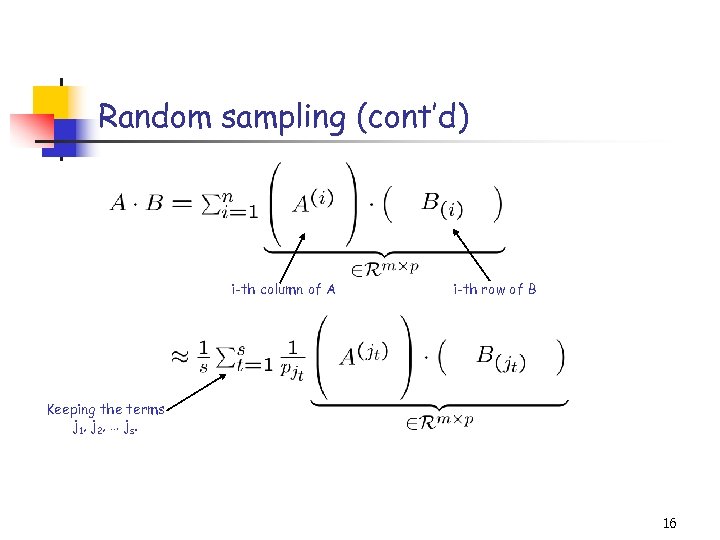Random sampling (cont’d) i-th column of A i-th row of B Keeping the terms j 1, j 2, … js. 16

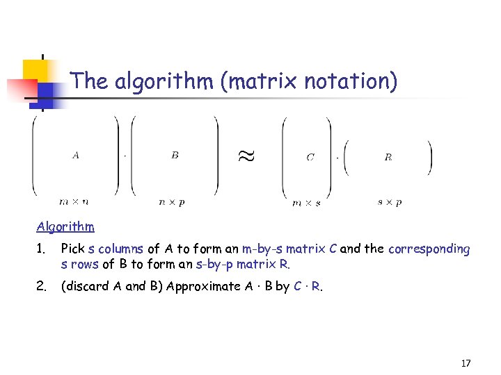The algorithm (matrix notation) Algorithm 1. Pick s columns of A to form an m-by-s matrix C and the corresponding s rows of B to form an s-by-p matrix R. 2. (discard A and B) Approximate A · B by C · R. 17

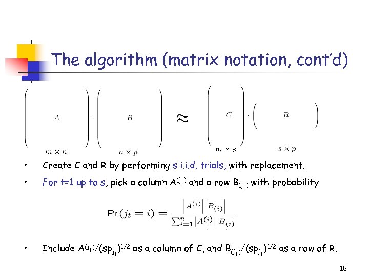The algorithm (matrix notation, cont’d) • Create C and R by performing s i. i. d. trials, with replacement. • For t=1 up to s, pick a column A(jt) and a row B(jt) with probability • Include A(jt)/(spjt)1/2 as a column of C, and B(jt)/(spjt)1/2 as a row of R. 18

Simple Lemmas The input matrices are given in “sparse unordered representation”; e. g. , their non-zero entries are presented as triples (i, j, Aij) in any order. • The expectation of CR (element-wise) is AB. • Our nonuniform sampling minimizes the variance of the estimator. • It is easy to implement the sampling in two passes. • If the matrices are dense the algorithm runs in O(smp) time, instead of O(nmp) time, • It requires O(sm+sp) RAM space. • Does not tamper with the sparsity of the matrices. 19

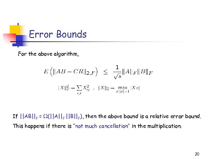Error Bounds For the above algorithm, If ||AB||F = (||A||F ||B||F), then the above bound is a relative error bound. This happens if there is “not much cancellation” in the multiplication. 20

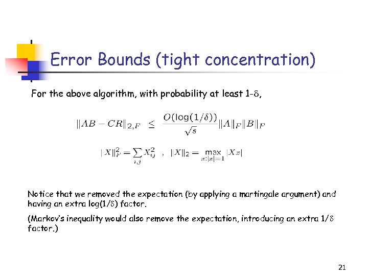Error Bounds (tight concentration) For the above algorithm, with probability at least 1 - , Notice that we removed the expectation (by applying a martingale argument) and having an extra log(1/ ) factor. (Markov’s inequality would also remove the expectation, introducing an extra 1/ factor. ) 21

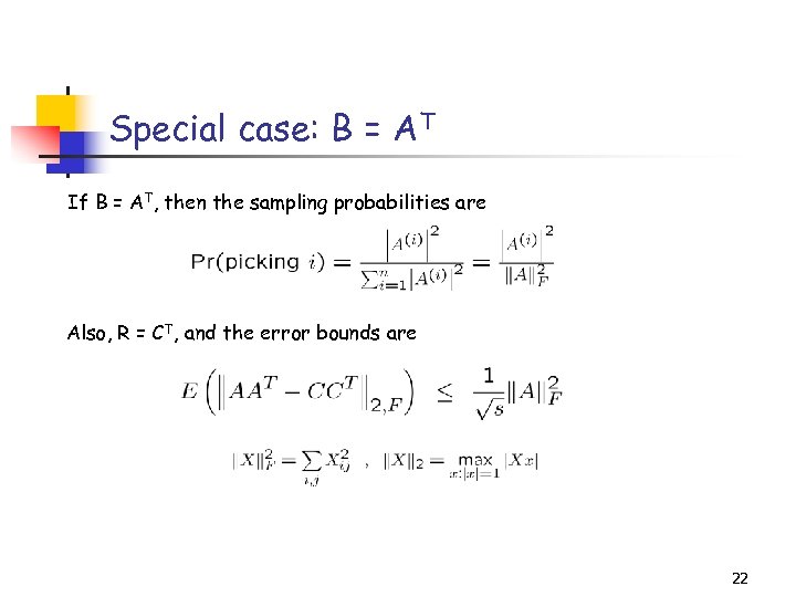Special case: B = AT If B = AT, then the sampling probabilities are Also, R = CT, and the error bounds are 22

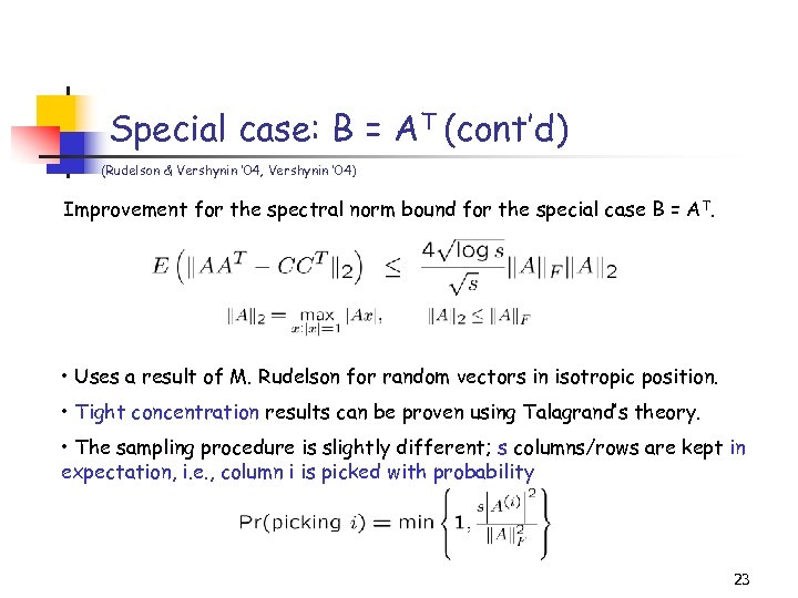Special case: B = AT (cont’d) (Rudelson & Vershynin ’ 04, Vershynin ’ 04) Improvement for the spectral norm bound for the special case B = A T. • Uses a result of M. Rudelson for random vectors in isotropic position. • Tight concentration results can be proven using Talagrand’s theory. • The sampling procedure is slightly different; s columns/rows are kept in expectation, i. e. , column i is picked with probability 23

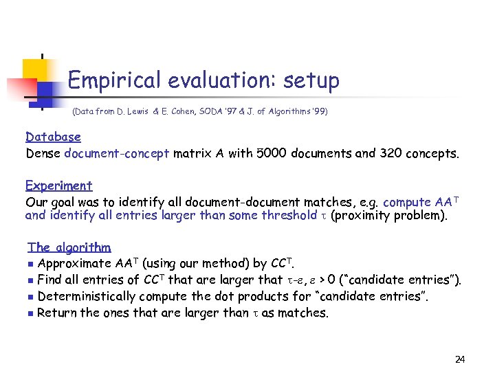Empirical evaluation: setup (Data from D. Lewis & E. Cohen, SODA ’ 97 & J. of Algorithms ’ 99) Database Dense document-concept matrix A with 5000 documents and 320 concepts. Experiment Our goal was to identify all document-document matches, e. g. compute AAT and identify all entries larger than some threshold (proximity problem). The algorithm n Approximate AAT (using our method) by CCT. n Find all entries of CCT that are larger that - , > 0 (“candidate entries”). n Deterministically compute the dot products for “candidate entries”. n Return the ones that are larger than as matches. 24

Empirical evaluation: results ( = 0. 85) 25

Empirical evaluation: results ( = 0. 75) 26

Experiments: uniform sampling 27

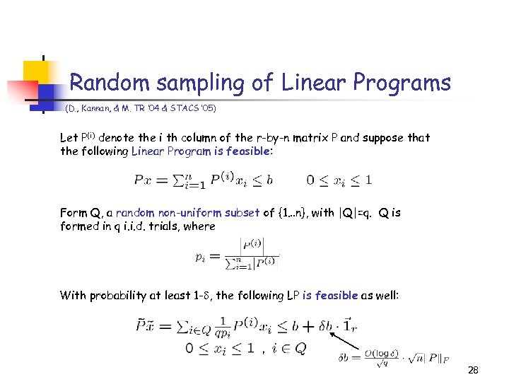Random sampling of Linear Programs (D. , Kannan, & M. TR ‘ 04 & STACS ’ 05) Let P(i) denote the i th column of the r-by-n matrix P and suppose that the following Linear Program is feasible: Form Q, a random non-uniform subset of {1…n}, with |Q|=q. Q is formed in q i. i. d. trials, where With probability at least 1 - , the following LP is feasible as well: 28

The picture … If feasible … Sample a few variables! …then feasible (with high probability). 29

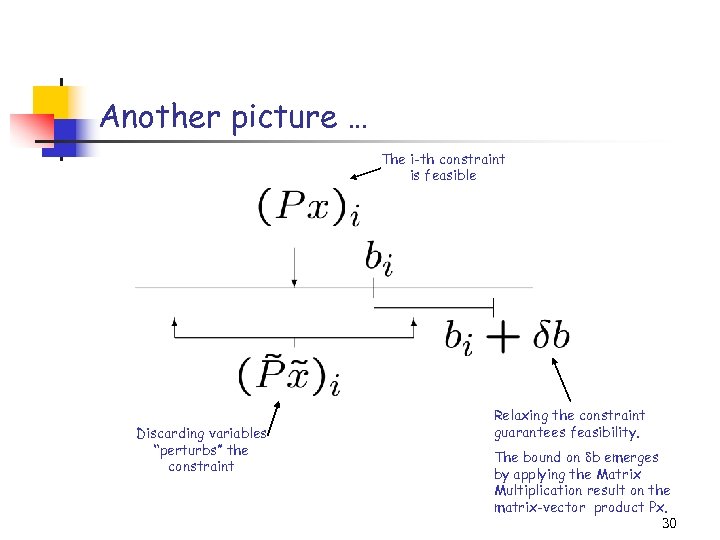Another picture … The i-th constraint is feasible Discarding variables “perturbs” the constraint Relaxing the constraint guarantees feasibility. The bound on b emerges by applying the Matrix Multiplication result on the matrix-vector product Px. 30

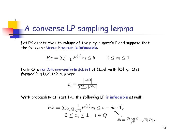A converse LP sampling lemma Let P(i) denote the i th column of the r-by-n matrix P and suppose that the following Linear Program is infeasible: Form Q, a random non-uniform subset of {1…n}, with |Q|=q. Q is formed in q i. i. d. trials, where With probability at least 1 - , the following LP is infeasible as well: 31

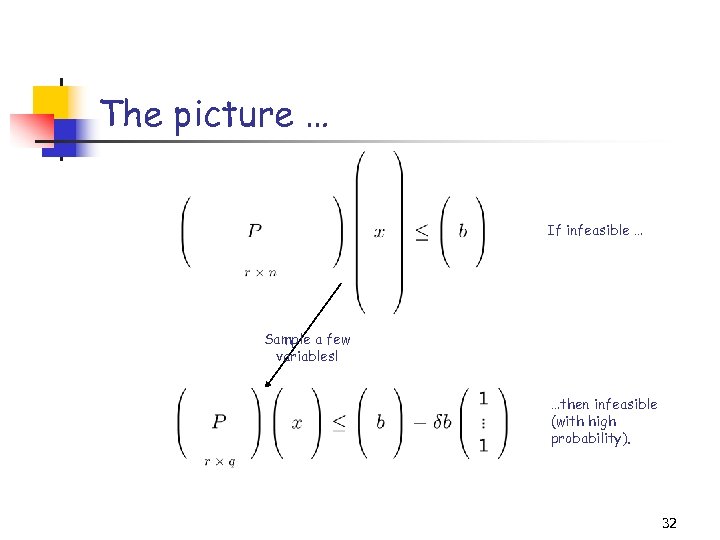The picture … If infeasible … Sample a few variables! …then infeasible (with high probability). 32

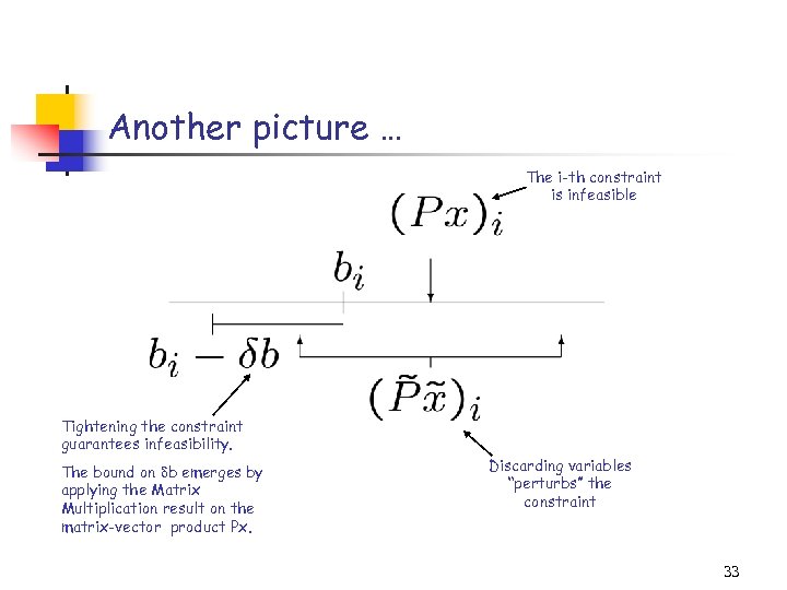Another picture … The i-th constraint is infeasible Tightening the constraint guarantees infeasibility. The bound on b emerges by applying the Matrix Multiplication result on the matrix-vector product Px. Discarding variables “perturbs” the constraint 33

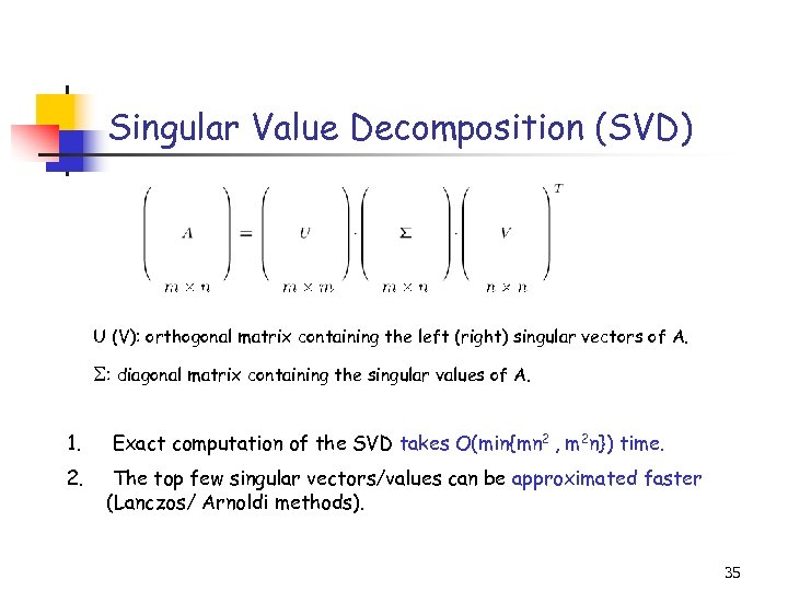Singular Value Decomposition (SVD) U (V): orthogonal matrix containing the left (right) singular vectors of A. : diagonal matrix containing the singular values of A. 1. Exact computation of the SVD takes O(min{mn 2 , m 2 n}) time. 2. The top few singular vectors/values can be approximated faster (Lanczos/ Arnoldi methods). 35

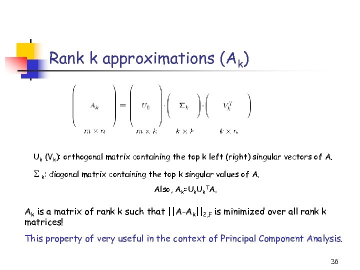Rank k approximations (Ak) Uk (Vk): orthogonal matrix containing the top k left (right) singular vectors of A. k: diagonal matrix containing the top k singular values of A. Also, Ak=Uk. TA. Ak is a matrix of rank k such that ||A-Ak||2, F is minimized over all rank k matrices! This property of very useful in the context of Principal Component Analysis. 36

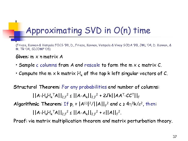Approximating SVD in O(n) time (Frieze, Kannan & Vempala FOCS ‘ 98, D. , Frieze, Kannan, Vempala & Vinay SODA ’ 99, JML ’ 04, D. Kannan, & M. TR ’ 04, SICOMP ’ 05) Given: m x n matrix A • Sample c columns from A and rescale to form the m x c matrix C. • Compute the m x k matrix Hk of the top k left singular vectors of C. Structural Theorem: For any probabilities and number of columns: ||A-Hk. TA||2, F 2 ≤ ||A-Ak||2, F 2 + 2√k||AAT-CCT||F Algorithmic Theorem: If pi = |A(i)|2/||A||F 2 and c ≥ 4 2 k/ 2, then: ||A-Hk. TA||2, F 2 ≤ ||A-Ak||2, F 2 + ||A||F 2. Proof: via matrix multiplication theorem and matrix perturbation theory. 37

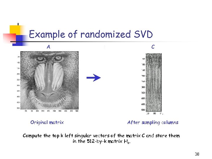Example of randomized SVD A C Title: C: PetrosImage Processingbaboondet. eps Creator: MATLAB, The Mathworks, Inc. Preview: This EPS picture was not saved with a preview included in it. Comment: This EPS picture will print to a Post. Script printer, but not to other types of printers. Original matrix After sampling columns Compute the top k left singular vectors of the matrix C and store them in the 512 -by-k matrix Hk. 38

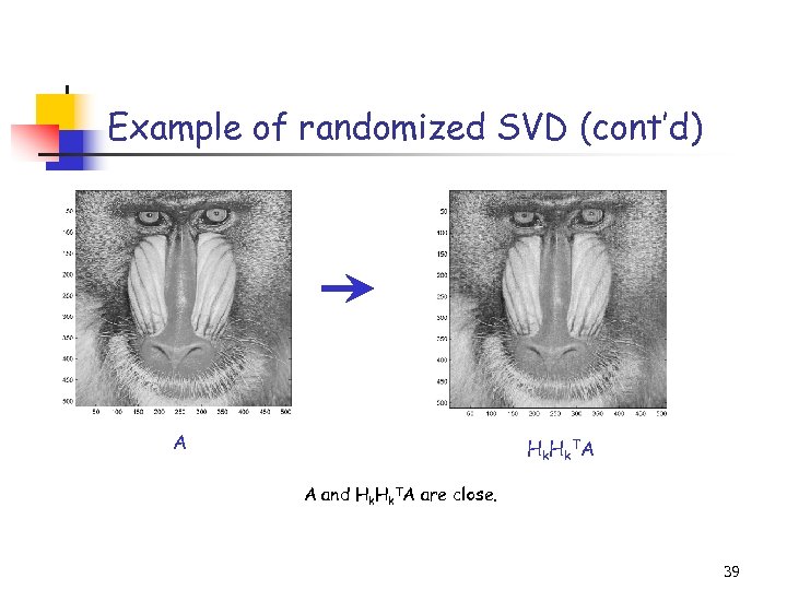Example of randomized SVD (cont’d) Title: C: PetrosImage Processingbaboondet. eps Creator: MATLAB, The Mathworks, Inc. Preview: This EPS picture was not saved with a preview included in it. Comment: This EPS picture will print to a Post. Script printer, but not to other types of printers. A Hk. TA A and Hk. TA are close. 39

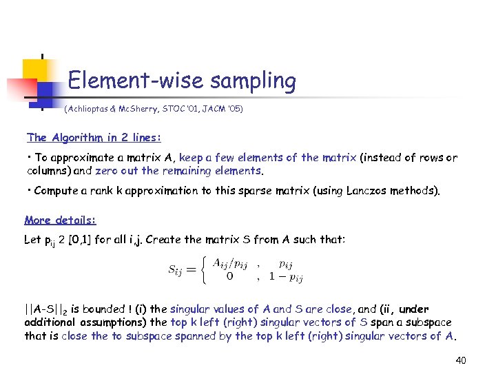Element-wise sampling (Achlioptas & Mc. Sherry, STOC ’ 01, JACM ’ 05) The Algorithm in 2 lines: • To approximate a matrix A, keep a few elements of the matrix (instead of rows or columns) and zero out the remaining elements. • Compute a rank k approximation to this sparse matrix (using Lanczos methods). More details: Let pij 2 [0, 1] for all i, j. Create the matrix S from A such that: ||A-S||2 is bounded ! (i) the singular values of A and S are close, and (ii, under additional assumptions) the top k left (right) singular vectors of S span a subspace that is close the to subspace spanned by the top k left (right) singular vectors of A. 40

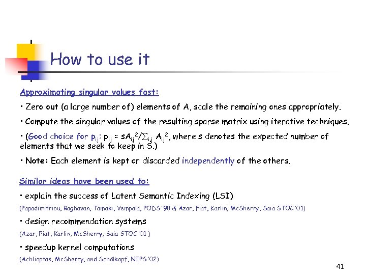How to use it Approximating singular values fast: • Zero out (a large number of) elements of A, scale the remaining ones appropriately. • Compute the singular values of the resulting sparse matrix using iterative techniques. • (Good choice for pij: pij = s. Aij 2/ i, j Aij 2, where s denotes the expected number of elements that we seek to keep in S. ) • Note: Each element is kept or discarded independently of the others. Similar ideas have been used to: • explain the success of Latent Semantic Indexing (LSI) (Papadimitriou, Raghavan, Tamaki, Vempala, PODS ’ 98 & Azar, Fiat, Karlin, Mc. Sherry, Saia STOC ’ 01) • design recommendation systems (Azar, Fiat, Karlin, Mc. Sherry, Saia STOC ’ 01 ) • speedup kernel computations (Achlioptas, Mc. Sherry, and Schölkopf, NIPS ’ 02) 41

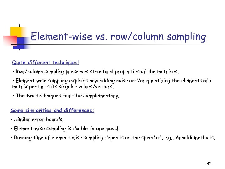Element-wise vs. row/column sampling Quite different techniques! • Row/column sampling preserves structural properties of the matrices. • Element-wise sampling explains how adding noise and/or quantizing the elements of a matrix perturbs its singular values/vectors. • The two techniques could be complementary! Some similarities and differences: • Similar error bounds. • Element-wise sampling is doable in one pass! • Running time of element-wise sampling depends on the speed of, e. g. , Arnoldi methods. 42

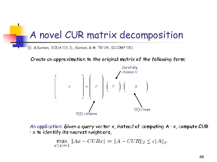A novel CUR matrix decomposition (D. & Kannan, SODA ’ 03, D. , Kannan, & M. TR ’ 04, SICOMP ’ 05) Create an approximation to the original matrix of the following form: Carefully chosen U O(1) columns O(1) rows An application: Given a query vector x, instead of computing A · x, compute CUR · x to identify its nearest neighbors, 44

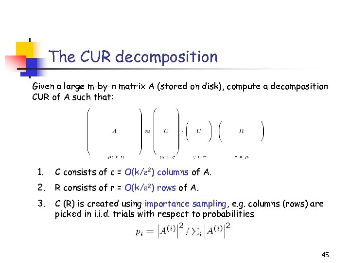The CUR decomposition Given a large m-by-n matrix A (stored on disk), compute a decomposition CUR of A such that: 1. C consists of c = O(k/ 2) columns of A. 2. R consists of r = O(k/ 2) rows of A. 3. C (R) is created using importance sampling, e. g. columns (rows) are picked in i. i. d. trials with respect to probabilities 45

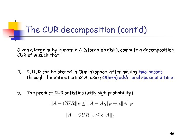The CUR decomposition (cont’d) Given a large m-by-n matrix A (stored on disk), compute a decomposition CUR of A such that: 4. C, U, R can be stored in O(m+n) space, after making two passes through the entire matrix A, using O(m+n) additional space and time. 5. The product CUR satisfies (with high probability) 46

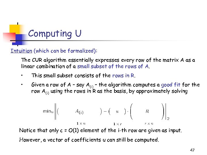Computing U Intuition (which can be formalized): The CUR algorithm essentially expresses every row of the matrix A as a linear combination of a small subset of the rows of A. • This small subset consists of the rows in R. • Given a row of A – say A(i) – the algorithm computes a good fit for the row A(i) using the rows in R as the basis, by approximately solving Notice that only c = O(1) element of the i-th row are given as input. However, a vector of coefficients u can still be computed. 47

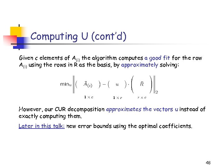Computing U (cont’d) Given c elements of A(i) the algorithm computes a good fit for the row A(i) using the rows in R as the basis, by approximately solving: However, our CUR decomposition approximates the vectors u instead of exactly computing them. Later in this talk: new error bounds using the optimal coefficients. 48

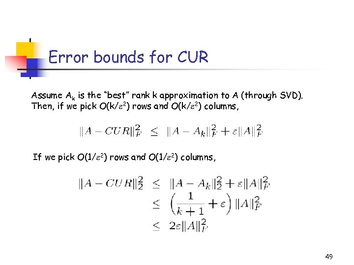Error bounds for CUR Assume Ak is the “best” rank k approximation to A (through SVD). Then, if we pick O(k/ 2) rows and O(k/ 2) columns, If we pick O(1/ 2) rows and O(1/ 2) columns, 49

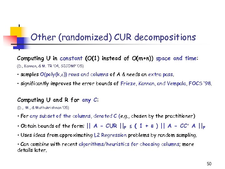Other (randomized) CUR decompositions Computing U in constant (O(1) instead of O(m+n)) space and time: (D. , Kannan, & M. TR ’ 04, SICOMP ’ 05) • samples O(poly(k, )) rows and columns of A & needs an extra pass. • significantly improves the error bounds of Frieze, Kannan, and Vempala, FOCS ’ 98. Computing U and R for any C: (D. , M. , & Muthukrishnan ’ 05) • For any subset of the columns, denoted C (e. g. , chosen by the practitioner) • Obtain bounds of the form: || A - CUR ||F ≤ ( 1 + ) || A - CC+ A ||F • Uses ideas from approximating L 2 Regression problems by random sampling. • Can combine with recent algorithms/heuristics for choosing columns; more details later. 50

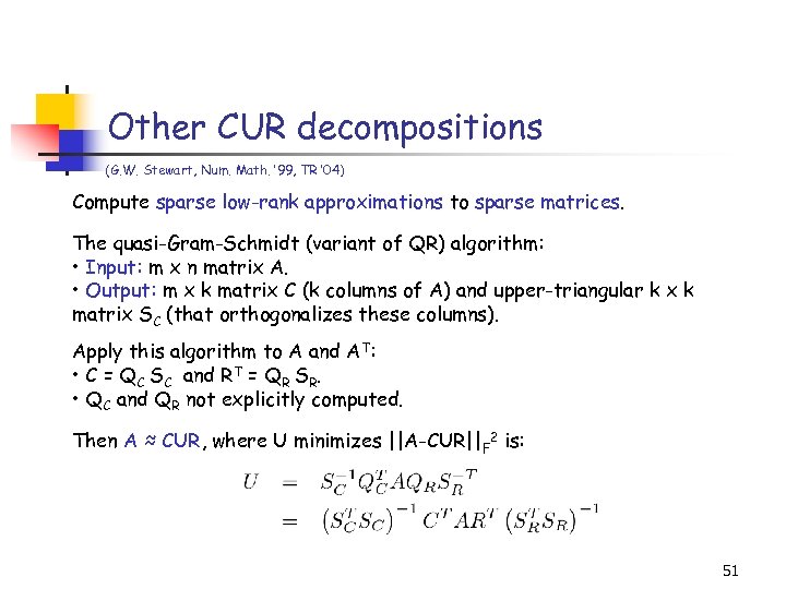Other CUR decompositions (G. W. Stewart, Num. Math. ’ 99, TR ’ 04) Compute sparse low-rank approximations to sparse matrices. The quasi-Gram-Schmidt (variant of QR) algorithm: • Input: m x n matrix A. • Output: m x k matrix C (k columns of A) and upper-triangular k x k matrix SC (that orthogonalizes these columns). Apply this algorithm to A and AT: • C = QC SC and RT = QR SR. • QC and QR not explicitly computed. Then A ≈ CUR, where U minimizes ||A-CUR||F 2 is: 51

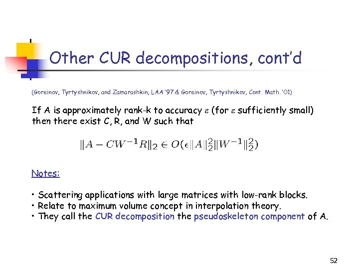Other CUR decompositions, cont’d (Goreinov, Tyrtyshnikov, and Zamarashkin, LAA ’ 97 & Goreinov, Tyrtyshnikov, Cont. Math. ’ 01) If A is approximately rank-k to accuracy (for sufficiently small) then there exist C, R, and W such that Notes: • Scattering applications with large matrices with low-rank blocks. • Relate to maximum volume concept in interpolation theory. • They call the CUR decomposition the pseudoskeleton component of A. 52

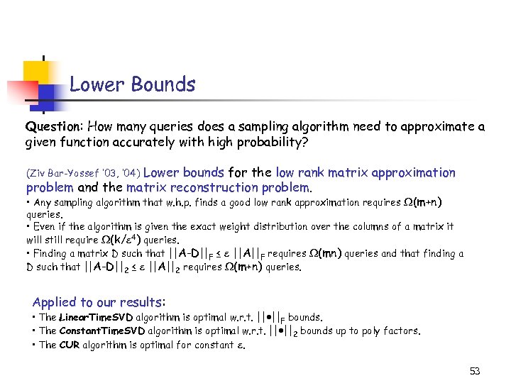Lower Bounds Question: How many queries does a sampling algorithm need to approximate a given function accurately with high probability? Lower bounds for the low rank matrix approximation problem and the matrix reconstruction problem. (Ziv Bar-Yossef ’ 03, ’ 04) • Any sampling algorithm that w. h. p. finds a good low rank approximation requires (m+n) queries. • Even if the algorithm is given the exact weight distribution over the columns of a matrix it will still require (k/ 4) queries. • Finding a matrix D such that ||A-D||F ≤ ||A||F requires (mn) queries and that finding a D such that ||A-D||2 ≤ ||A||2 requires (m+n) queries. Applied to our results: • The Linear. Time. SVD algorithm is optimal w. r. t. || ||F bounds. • The Constant. Time. SVD algorithm is optimal w. r. t. || ||2 bounds up to poly factors. • The CUR algorithm is optimal for constant . 53

Approximating Max-Cut (NP-hard for general and dense graphs, Max-SNP) Given a graph G=(V, E), |V|=n, partition V in two disjoint subsets V 1 and V 2 such that the number of edges of E that have one endpoint in V 1 and one endpoint in V 2 is maximized. Goemans & Williamson ’ 94: . 878 -approximation algorithm (might be tight!) Arora, Karger & Karpinski ’ 95: LP based, n 2 additive error(*) De La Vega ’ 96: Combinatorial methods, n 2 additive error Frieze & Kannan ’ 96: Linear Algebraic methods, n 2 additive error(*) Goldreich, Goldwasser & Ron ’ 96: Property Testing, n 2 additive error Alon, De La Vega, Kannan & Karpinski ’ 02, ’ 03 : Cut Decomposition, n 2 additive error(*) All the above algorithms run in constant time/space. (*) More generally, it achieves nr for all problems in Max-r-CSP (=Max-SNP) 55

Weighted Max-Cut via CUR (D. , Kannan, & M. TR ’ 04 and STACS ’ 05) Let A denote the adjacency matrix of G. All previous algorithms also guarantee an additive error approximation for the weighted Max-Cut problem, where Amax is the maximum edge weight in the graph. Our result: We can approximate the weighted Max-Cut of G(V, E) up to additive error in constant time and space after reading the graph a small number of times. 56

The algorithm (sketch) Let A denote the adjacency matrix of the weighted graph G=(V, E). Then, Step 1: Replace A by the Constant. Time. CUR decomposition. Then, Follows from Compute the Max. Cut of CUR, thus getting an approximation to the Max. Cut of A. It turns out that we can solve the problem on CUR in constant time, in constant space… 57

Data mining with CUR We are given m (>106) objects and n(>105) features describing the objects. Database An m-by-n matrix A (Aij shows the “importance” of feature j for object i). E. g. , m documents, represented w. r. t. n terms. Queries Given a new object x, find similar objects in the database (nearest neighbors). 58

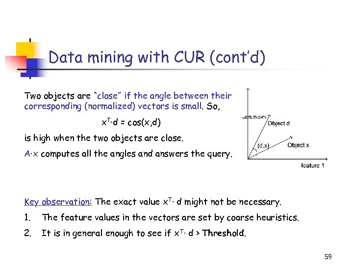Data mining with CUR (cont’d) Two objects are “close” if the angle between their corresponding (normalized) vectors is small. So, x. T·d = cos(x, d) is high when the two objects are close. A·x computes all the angles and answers the query. Key observation: The exact value x. T· d might not be necessary. 1. The feature values in the vectors are set by coarse heuristics. 2. It is in general enough to see if x. T· d > Threshold. 59

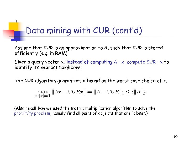Data mining with CUR (cont’d) Assume that CUR is an approximation to A, such that CUR is stored efficiently (e. g. in RAM). Given a query vector x, instead of computing A · x, compute CUR · x to identify its nearest neighbors. The CUR algorithm guarantees a bound on the worst case choice of x. (Also recall how we used the matrix multiplication algorithm to solve the proximity problem, namely find all pairs of objects that are “close”. ) 60

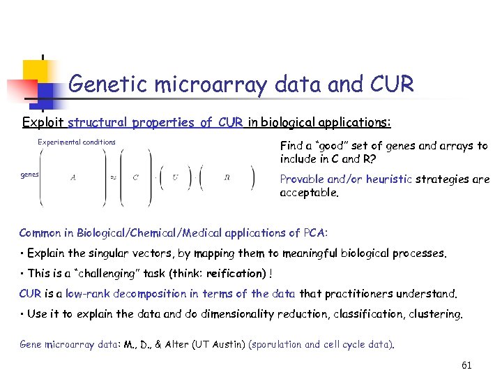Genetic microarray data and CUR Exploit structural properties of CUR in biological applications: Experimental conditions genes Find a “good” set of genes and arrays to include in C and R? Provable and/or heuristic strategies are acceptable. Common in Biological/Chemical/Medical applications of PCA: • Explain the singular vectors, by mapping them to meaningful biological processes. • This is a “challenging” task (think: reification) ! CUR is a low-rank decomposition in terms of the data that practitioners understand. • Use it to explain the data and do dimensionality reduction, classification, clustering. Gene microarray data: M. , D. , & Alter (UT Austin) (sporulation and cell cycle data). 61

Recommendation Systems (D. , Raghavan, & Kerenidis, STOC ’ 02) The problem: Assume the existence of m customers and n products. Then, A is an (unknown) matrix s. t. Aij is the utility of product j for customer i. Our goal is to recreate A from a few samples, s. t. we can recommend high utility products to customers. • (Kumar, Raghavan, Rajagopalan & Tomkins FOCS ’ 98) Assuming strong clustering of the products, they offer competitive algorithms even with only 2 samples/customer. • (Azar, Fiat, Karlin, Mc. Sherry & Saia STOC ’ 01) Assuming sampling of (mn) entries of A and a certain gap requirement, they -veryaccurately recreate A. 62

Recommendation Systems The problem: Assume the existence of m customers and n products. Then, A is an (unknown) matrix s. t. Aij is the utility of product j for customer i. Our goal is to recreate A from a few samples, s. t. we can recommend high utility products to customers. Critical assumption (supported by experimental evidence): There exist a small, constant (e. g. k) number of different customer types or, equivalently, the rows of the matrix A are (approximately) linearly dependent or, equivalently, the matrix A has a “good” low-rank (e. g. k) approximation. 63

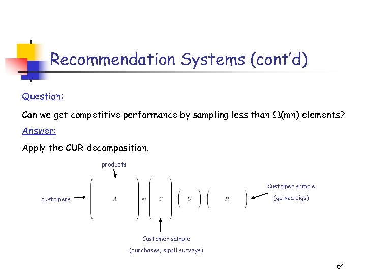Recommendation Systems (cont’d) Question: Can we get competitive performance by sampling less than (mn) elements? Answer: Apply the CUR decomposition. products Customer sample (guinea pigs) customers Customer sample (purchases, small surveys) 64

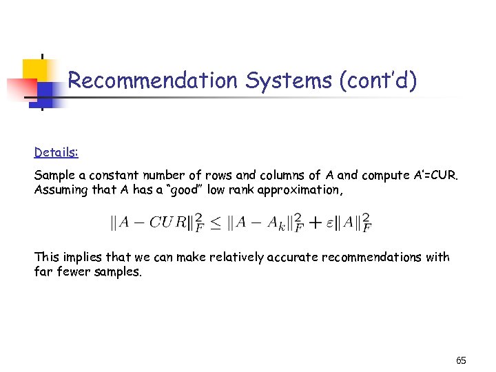Recommendation Systems (cont’d) Details: Sample a constant number of rows and columns of A and compute A’=CUR. Assuming that A has a “good” low rank approximation, This implies that we can make relatively accurate recommendations with far fewer samples. 65

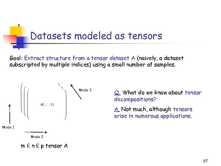Datasets modeled as tensors Goal: Extract structure from a tensor dataset A (naively, a dataset subscripted by multiple indices) using a small number of samples. Mode 3 Q. What do we know about tensor decompositions? A. Not much, although tensors arise in numerous applications. Mode 1 Mode 2 m £ n £ p tensor A 67

Tensors in Applications Tensors appear both in Math and CS. • Represent high dimensional functions. • Connections to complexity theory (i. e. , matrix multiplication complexity). • Statistical applications (i. e. , Independent Component Analysis, higher order statistics, etc. ). • Large data-set applications (e. g. , Medical Imaging & Hyperspectral Imaging) Problem: There does not exist a definition of tensor rank (and associated tensor SVD) with the – nice – properties found in the matrix case. (Lek-Heng Lim ’ 05: strong impossibility results!) Heuristic solution: “unfold” the tensor along a mode and apply Linear Algebra. 68

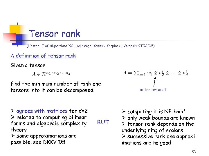Tensor rank (Hastad, J of Algorithms ’ 90, De. La. Vega, Kannan, Karpinski, Vempala STOC ’ 05) A definition of tensor rank Given a tensor find the minimum number of rank one tensors into it can be decomposed. Ø agrees with matrices for d=2 Ø related to computing bilinear forms and algebraic complexity theory Ø some approximations are possible, see DKKV ’ 05 BUT outer product Ø computing it is NP-hard Ø only weak bounds are known Ø tensor rank depends on the underlying ring of scalars Ø successive rank one approxiimations are no good 69

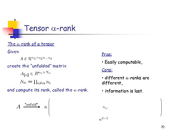Tensor -rank The -rank of a tensor Given Pros: create the “unfolded” matrix • Easily computable, Cons: • different -ranks are different, and compute its rank, called the -rank. • information is lost. “unfold” 70

Tensors in real applications 3 classes of tensors in data applications 1. All modes are comparable (e. g. , tensor faces, chemometrics) 2. A priori dominant mode (e. g. , coarse scales, microarrays vs. time, images vs. frequency) 3. All other combinations (D. and M. ’ 05) Tensor. SVD paper deals with (1). We will focus on (2), where there is a preferred mode. 71

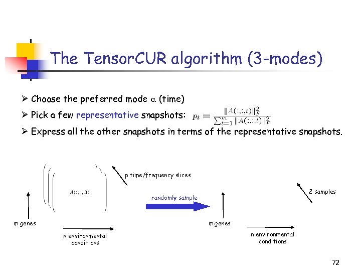The Tensor. CUR algorithm (3 -modes) Ø Choose the preferred mode (time) Ø Pick a few representative snapshots: Ø Express all the other snapshots in terms of the representative snapshots. p time/frequency slices 2 samples randomly sample m genes n environmental conditions 72

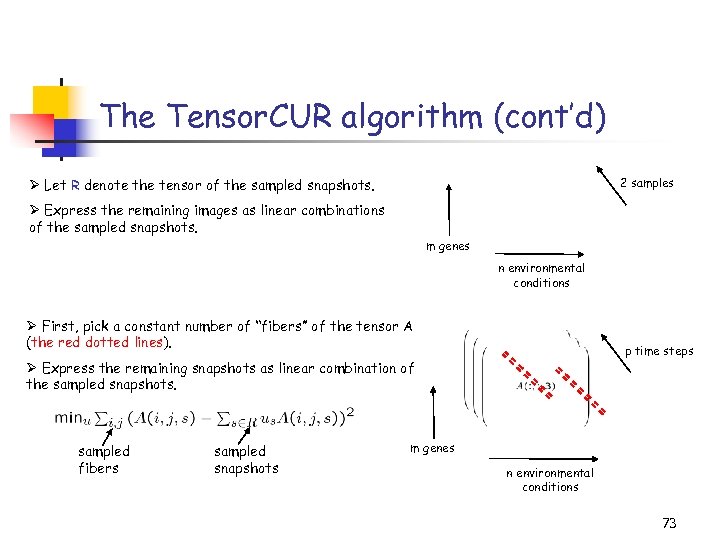The Tensor. CUR algorithm (cont’d) 2 samples Ø Let R denote the tensor of the sampled snapshots. Ø Express the remaining images as linear combinations of the sampled snapshots. m genes n environmental conditions Ø First, pick a constant number of “fibers” of the tensor A (the red dotted lines). p time steps Ø Express the remaining snapshots as linear combination of the sampled snapshots. sampled fibers sampled snapshots m genes n environmental conditions 73

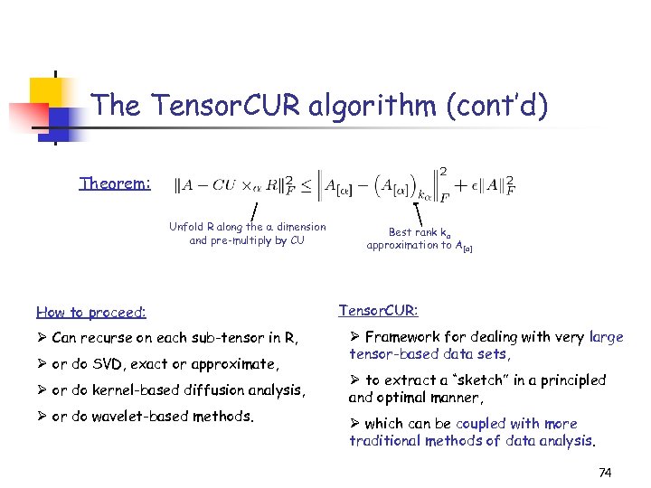The Tensor. CUR algorithm (cont’d) Theorem: Unfold R along the dimension and pre-multiply by CU How to proceed: Ø Can recurse on each sub-tensor in R, Ø or do SVD, exact or approximate, Ø or do kernel-based diffusion analysis, Ø or do wavelet-based methods. Best rank ka approximation to A[a] Tensor. CUR: Ø Framework for dealing with very large tensor-based data sets, Ø to extract a “sketch” in a principled and optimal manner, Ø which can be coupled with more traditional methods of data analysis. 74

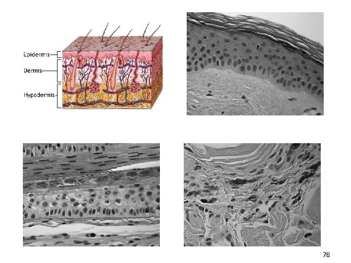
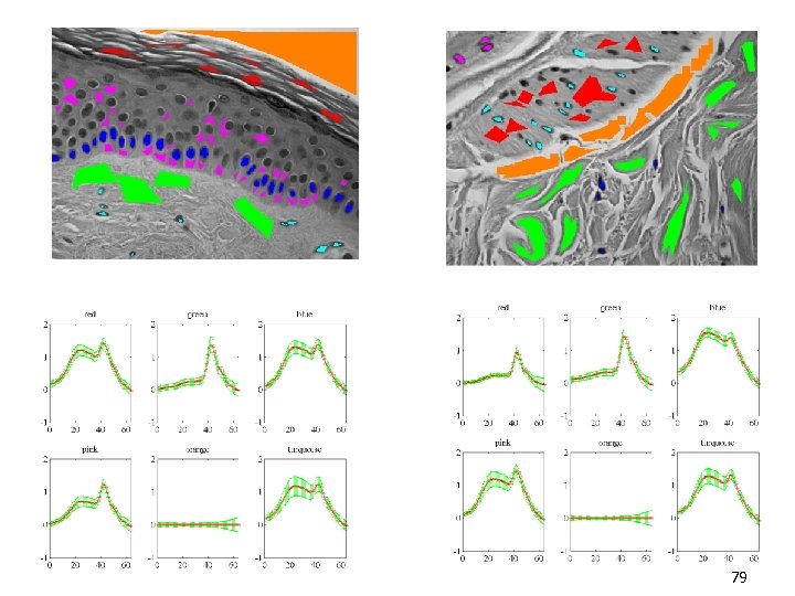
Tensor. CUR on scientific data sets Apply random sampling methodology and kernel-based Laplacian methods to large physical and chemical and biological data sets. Common application areas of large data set analysis: • telecommunications, • finance, • web-based modeling, and • astronomy. Scientific data sets are quite different: • with respect to their size, • with respect to their noise properties, and • with respect to the available field-specific intuition. 76

Data sets being considered Sequence and mutational data from G-protein coupled receptors • to identify mutants with enhanced stability properties. Genomic microarray data • to understand large-scale genomic and cellular behavior. Hyperspectral colon cancer data • for improved detection of anomalous behavior. Time-resolved f. MRI data • to better represent large, complex visual brain-imaging data. Simulational data • to more efficiently conduct large scale computations. 77

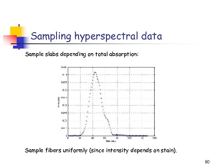Sampling hyperspectral data Sample slabs depending on total absorption: Sample fibers uniformly (since intensity depends on stain). 80

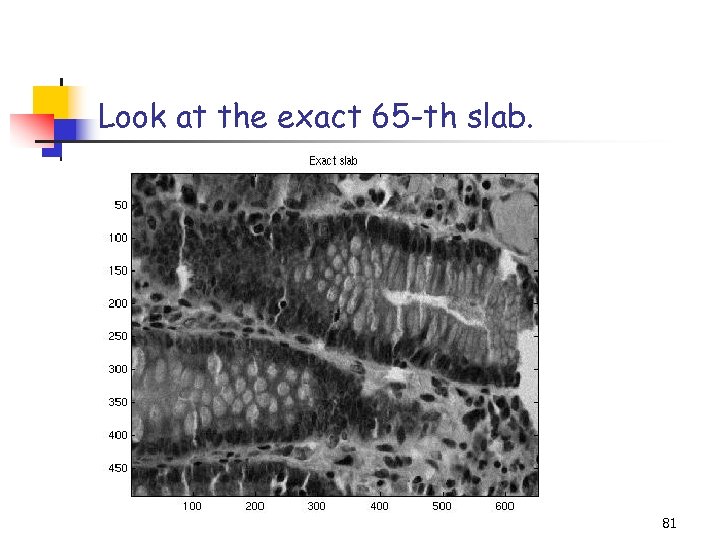Look at the exact 65 -th slab. 81

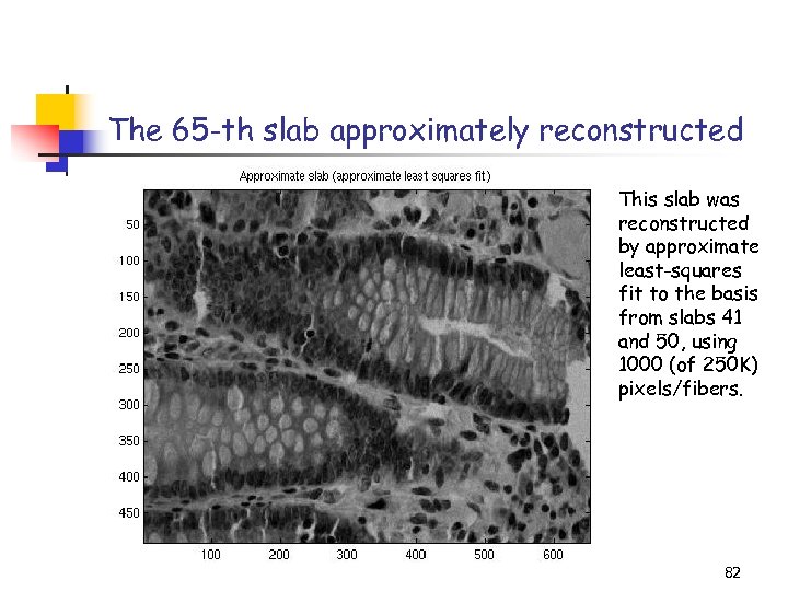The 65 -th slab approximately reconstructed This slab was reconstructed by approximate least-squares fit to the basis from slabs 41 and 50, using 1000 (of 250 K) pixels/fibers. 82

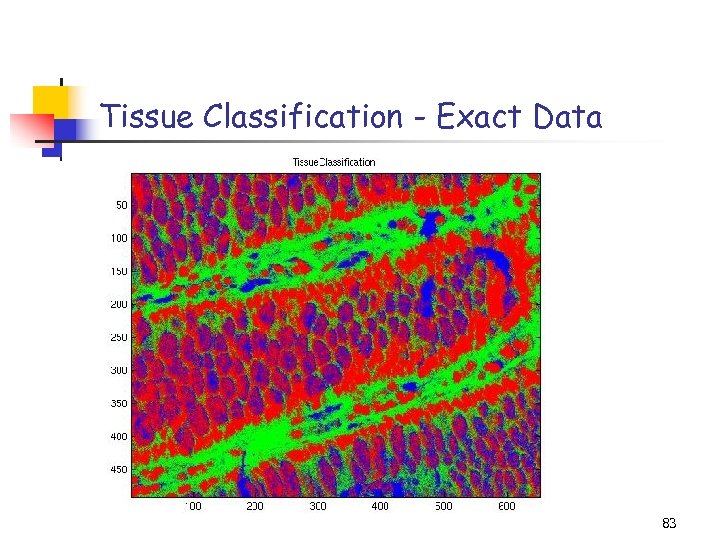Tissue Classification - Exact Data 83

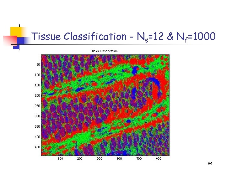Tissue Classification - Ns=12 & Nf=1000 84

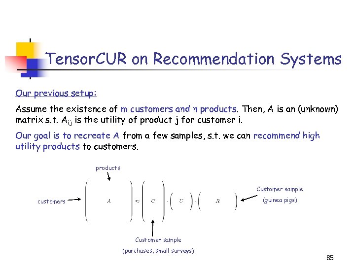Tensor. CUR on Recommendation Systems Our previous setup: Assume the existence of m customers and n products. Then, A is an (unknown) matrix s. t. Aij is the utility of product j for customer i. Our goal is to recreate A from a few samples, s. t. we can recommend high utility products to customers. products Customer sample (guinea pigs) customers Customer sample (purchases, small surveys) 85

Recommendation Systems (cont’d) Comment: It is folklore knowledge in economics literature that product utility is an ordinal and not a cardinal quantity. Thus, it is more natural to compare products than assign utility values. Model revisited: Every customer has an n-by-n matrix (whose entries are § 1) and represent pairwise product comparisons. Overall, there are m such matrices, forming an n-by-m 3 -mode array or a three-dimensional tensor, denoted by A. We seek to extract the “structure” of this tensor by sampling. 86

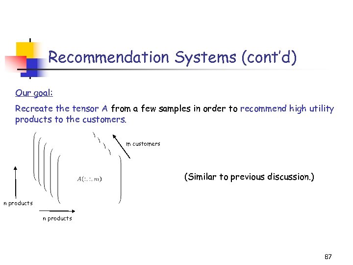Recommendation Systems (cont’d) Our goal: Recreate the tensor A from a few samples in order to recommend high utility products to the customers. m customers (Similar to previous discussion. ) n products 87

Motivation for Kernels (1 of 3) Methods to extract linear structure from the data: • Support Vector Machines (SVMs). • Gaussian Processes (GPs). • Singular Value Decomposition (SVD) and the related PCA. Kernel-based learning methods to extract non-linear structure: • Choose features to define a (dot product) space F. • Map the data, X, to F by : X ! F. • Do classification, regression, and clustering in F with linear methods. 89

Motivation for Kernels (2 of 3) • Use dot products for information about mutual positions. • Define the kernel or Gram matrix: Gij=kij=( (X(i)), (X(j))). • Algorithms that are expressed in terms of dot products may be given as input the Gram matrix G instead of the data covariance matrix XTX. Note: Isomap, LLE, graph Laplacian eigenmaps, Hessian eigenmaps, SDE (dimensionality reduction methods for nonlinear manifolds) are kernel-PCA for particular Gram matrices. Note: for Mercer kernels, G is SPSD. 90

Motivation for Kernels (3 of 3) If the Gram matrix G, where Gij=kij=( (X(i)), (X(j))), is dense but has low numerical rank, then calculations of interest still need O(n 2) space and O(n 3) time: • matrix inversion in GP prediction, • quadratic programming problems in SVMs, • computation of eigendecomposition of G. Relevant recent work using low-rank methods: • (Achlioptas, Mc. Sherry, and Schölkopf, NIPS ’ 02), randomized kernels. • Nystrom method for out-of-sample extensions NIPS ’ 01 and others), . (Williams and Seeger, 91

Kernel-CUR (D. & M. , COLT ’ 05, TR ’ 05) Main algorithm: • Randomized algorithm to approximate a Gram matrix. • Low-rank approximation in terms of columns (and rows) of G=X TX. Main quality-of-approximation theorem: • Provably good approximation if nonuniform probabilities are used. Discussion of the Nystrom method: • Nystrom method for integral equations and matrix problems. • Relationship to randomized SVD and CUR algorithms. 92

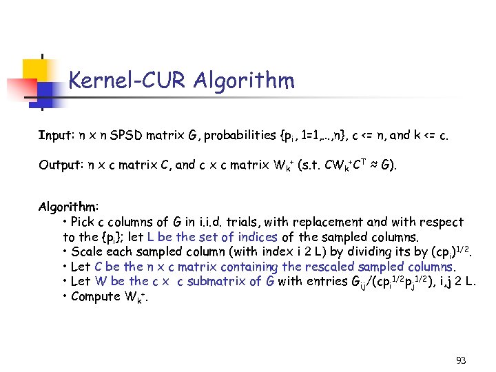Kernel-CUR Algorithm Input: n x n SPSD matrix G, probabilities {pi, 1=1, …, n}, c <= n, and k <= c. Output: n x c matrix C, and c x c matrix Wk+ (s. t. CWk+CT ≈ G). Algorithm: • Pick c columns of G in i. i. d. trials, with replacement and with respect to the {pi}; let L be the set of indices of the sampled columns. • Scale each sampled column (with index i 2 L) by dividing its by (cpi)1/2. • Let C be the n x c matrix containing the rescaled sampled columns. • Let W be the c x c submatrix of G with entries Gij/(cpi 1/2 pj 1/2), i, j 2 L. • Compute Wk+. 93

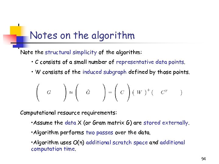Notes on the algorithm Note the structural simplicity of the algorithm: • C consists of a small number of representative data points. • W consists of the induced subgraph defined by those points. Computational resource requirements: • Assume the data X (or Gram matrix G) are stored externally. • Algorithm performs two passes over the data. • Algorithm uses O(n) additional scratch space and additional computation time. 94

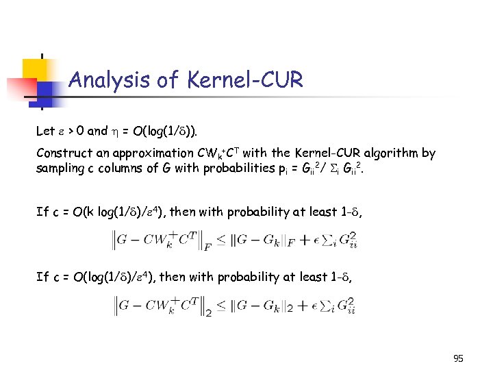Analysis of Kernel-CUR Let > 0 and = O(log(1/ )). Construct an approximation CWk+CT with the Kernel-CUR algorithm by sampling c columns of G with probabilities pi = Gii 2/ i Gii 2. If c = O(k log(1/ )/ 4), then with probability at least 1 - , If c = O(log(1/ )/ 4), then with probability at least 1 - , 95

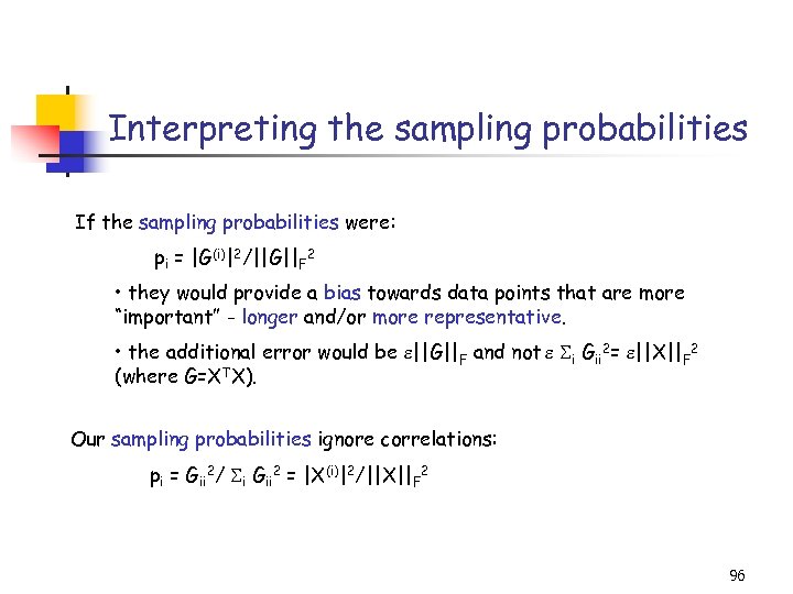Interpreting the sampling probabilities If the sampling probabilities were: pi = |G(i)|2/||G||F 2 • they would provide a bias towards data points that are more “important” - longer and/or more representative. • the additional error would be ||G||F and not i Gii 2= ||X||F 2 (where G=XTX). Our sampling probabilities ignore correlations: pi = Gii 2/ i Gii 2 = |X(i)|2/||X||F 2 96

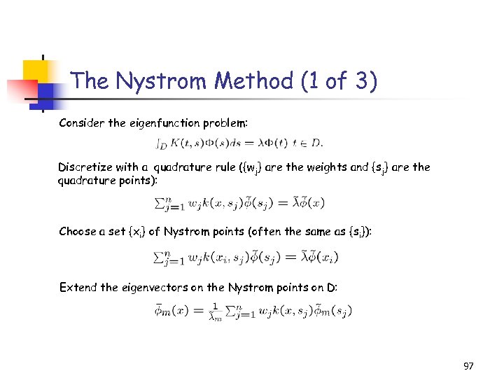The Nystrom Method (1 of 3) Consider the eigenfunction problem: Discretize with a quadrature rule ({wj} are the weights and {sj} are the quadrature points): Choose a set {xi} of Nystrom points (often the same as {si}): Extend the eigenvectors on the Nystrom points on D: 97

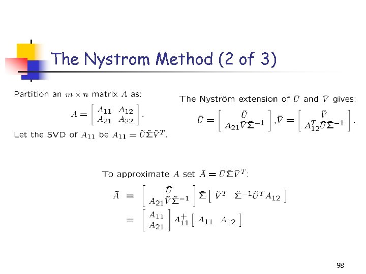The Nystrom Method (2 of 3) 98

The Nystrom Method (3 of 3) Randomized SVD Algorithms • Randomly sample columns (or rows). • Compute/approximate low-dimensional singular vectors. • Nystrom-extend to approximate Hk, the high-dimensional singular vectors. • Bound ||A-Hk. TA||2, F <= ||A-Ak||2, F + ||A||F. Randomized CUR Algorithms • Randomly sample columns and rows. • Bound ||A-CUR||2, F <= ||A-Ak||2, F + ||A||F. • Do not need or use the SPSD property. 99

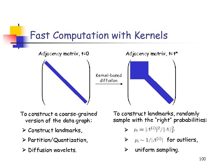Fast Computation with Kernels Adjacency matrix, t=0 Adjacency matrix, t=t* Kernel-based diffusion To construct a coarse-grained version of the data graph: To construct landmarks, randomly sample with the “right” probabilities: Ø Construct landmarks, Ø Ø Partition/Quantization, Ø Ø Diffusion wavelets. Ø for outliers, uniform sampling. 100

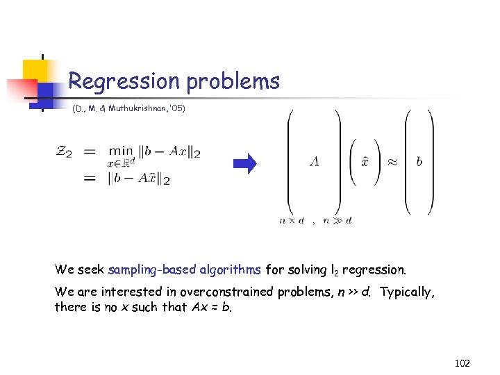Regression problems (D. , M. & Muthukrishnan, ’ 05) We seek sampling-based algorithms for solving l 2 regression. We are interested in overconstrained problems, n >> d. Typically, there is no x such that Ax = b. 102

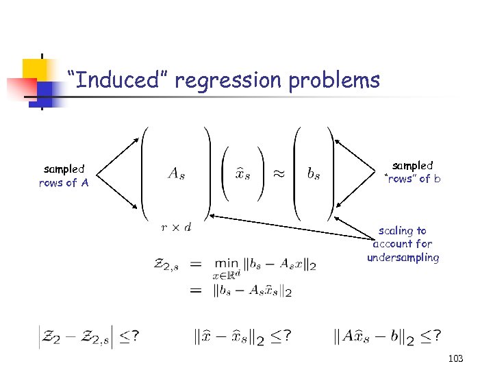“Induced” regression problems sampled rows of A sampled “rows” of b scaling to account for undersampling 103

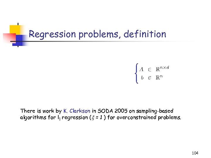Regression problems, definition There is work by K. Clarkson in SODA 2005 on sampling-based algorithms for l 1 regression ( = 1 ) for overconstrained problems. 104

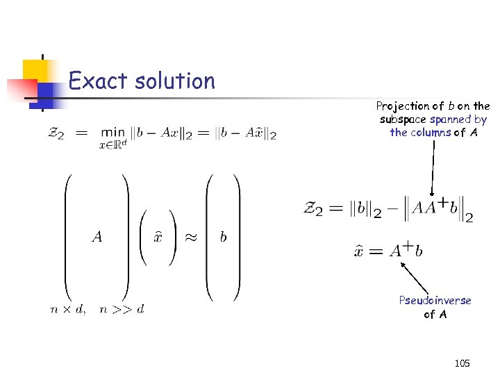Exact solution Projection of b on the subspace spanned by the columns of A Pseudoinverse of A 105

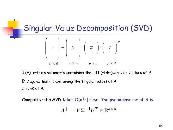Singular Value Decomposition (SVD) U (V): orthogonal matrix containing the left (right) singular vectors of A. : diagonal matrix containing the singular values of A. : rank of A. Computing the SVD takes O(d 2 n) time. The pseudoinverse of A is 106

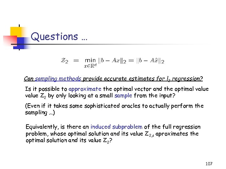Questions … Can sampling methods provide accurate estimates for l 2 regression? Is it possible to approximate the optimal vector and the optimal value Z 2 by only looking at a small sample from the input? (Even if it takes some sophisticated oracles to actually perform the sampling …) Equivalently, is there an induced subproblem of the full regression problem, whose optimal solution and its value Z 2, s aproximates the optimal solution and its value Z 2? 107

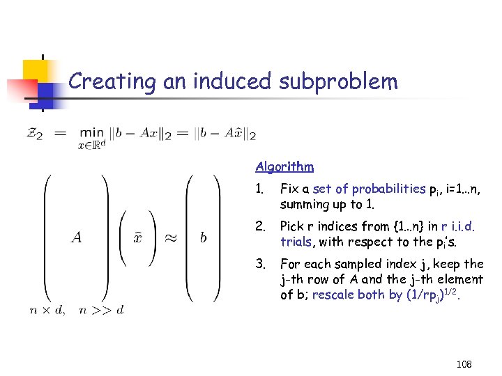Creating an induced subproblem Algorithm 1. Fix a set of probabilities pi, i=1…n, summing up to 1. 2. Pick r indices from {1…n} in r i. i. d. trials, with respect to the pi’s. 3. For each sampled index j, keep the j-th row of A and the j-th element of b; rescale both by (1/rpj)1/2. 108

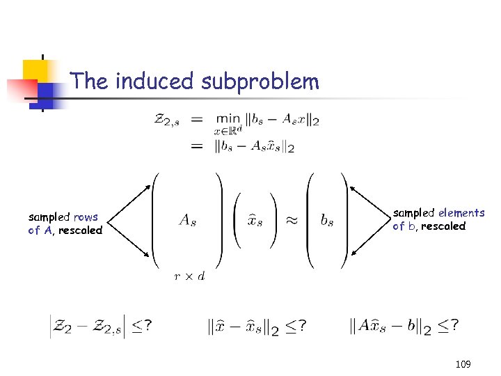The induced subproblem sampled rows of A, rescaled sampled elements of b, rescaled 109

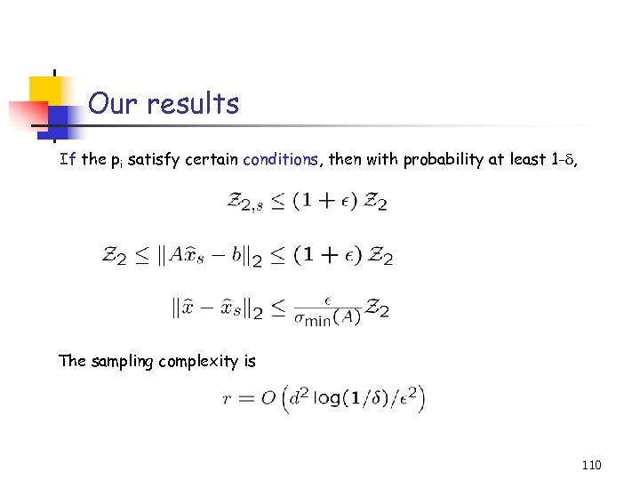Our results If the pi satisfy certain conditions, then with probability at least 1 - , The sampling complexity is 110

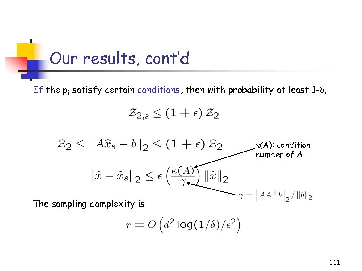Our results, cont’d If the pi satisfy certain conditions, then with probability at least 1 - , (A): condition number of A The sampling complexity is 111

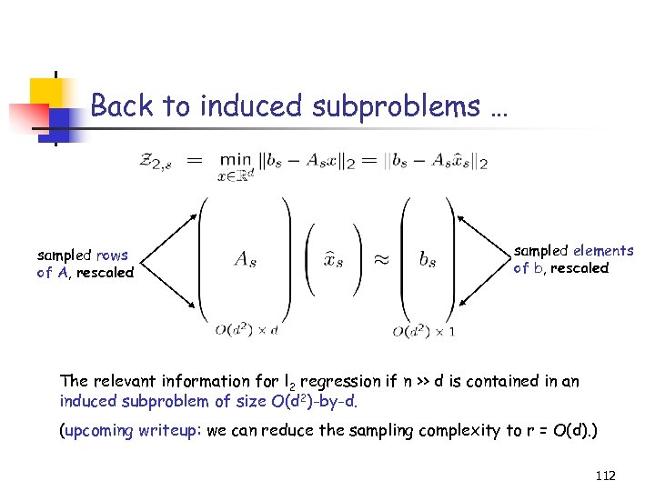Back to induced subproblems … sampled rows of A, rescaled sampled elements of b, rescaled The relevant information for l 2 regression if n >> d is contained in an induced subproblem of size O(d 2)-by-d. (upcoming writeup: we can reduce the sampling complexity to r = O(d). ) 112

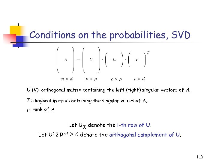Conditions on the probabilities, SVD U (V): orthogonal matrix containing the left (right) singular vectors of A. : diagonal matrix containing the singular values of A. : rank of A. Let U(i) denote the i-th row of U. Let U? 2 Rn £ (n - ) denote the orthogonal complement of U. 113

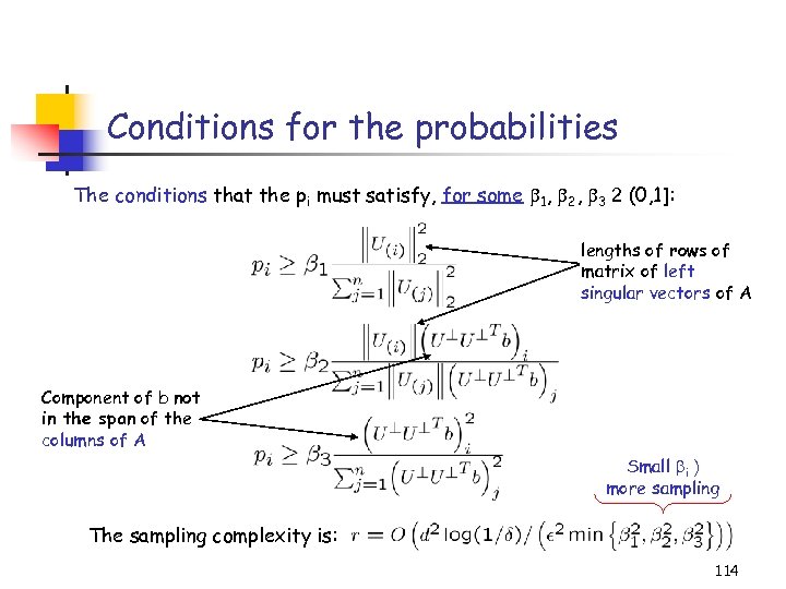Conditions for the probabilities The conditions that the pi must satisfy, for some 1, 2, 3 2 (0, 1]: lengths of rows of matrix of left singular vectors of A Component of b not in the span of the columns of A Small i ) more sampling The sampling complexity is: 114

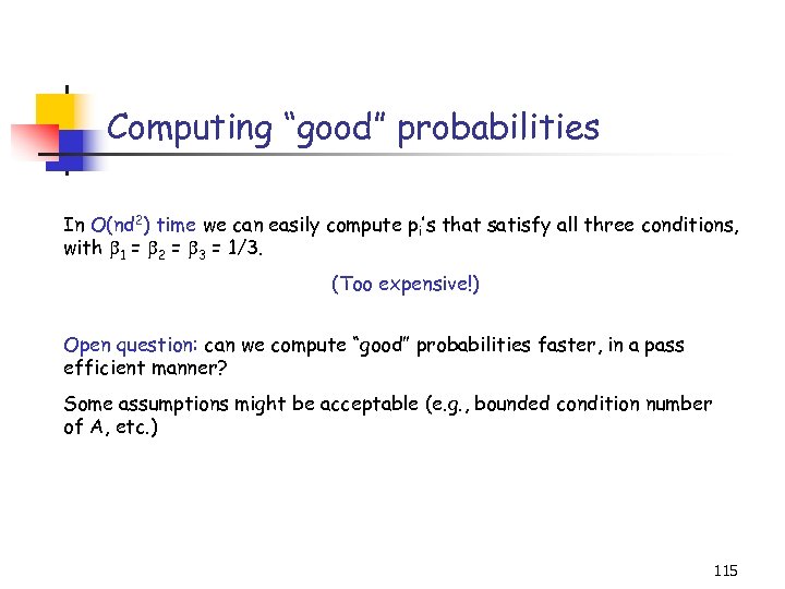Computing “good” probabilities In O(nd 2) time we can easily compute pi’s that satisfy all three conditions, with 1 = 2 = 3 = 1/3. (Too expensive!) Open question: can we compute “good” probabilities faster, in a pass efficient manner? Some assumptions might be acceptable (e. g. , bounded condition number of A, etc. ) 115

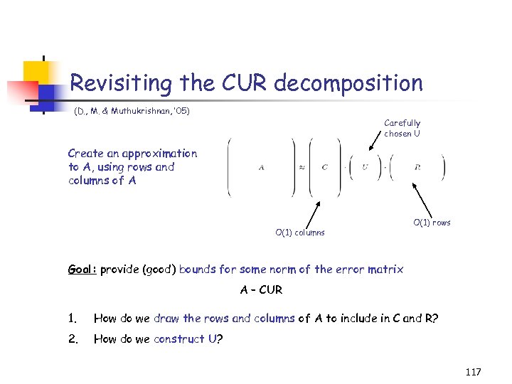Revisiting the CUR decomposition (D. , M. & Muthukrishnan, ’ 05) Carefully chosen U Create an approximation to A, using rows and columns of A O(1) columns O(1) rows Goal: provide (good) bounds for some norm of the error matrix A – CUR 1. How do we draw the rows and columns of A to include in C and R? 2. How do we construct U? 117

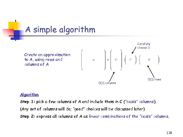A simple algorithm Carefully chosen U Create an approximation to A, using rows and columns of A O(1) columns O(1) rows Algorithm Step 1: pick a few columns of A and include them in C (“basis” columns). (Any set of columns will do; “good” choices will be discussed later) Step 2: express all columns of A as linear combinations of the “basis” columns. 118

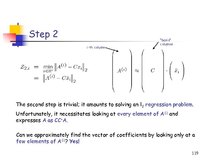Step 2 i-th column “basis” columns The second step is trivial; it amounts to solving an l 2 regression problem. Unfortunately, it necessitates looking at every element of A(i) and expresses A as CC+A. Can we approximately find the vector of coefficients by looking only at a few elements of A(i)? Yes! 119

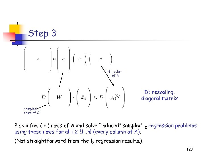Step 3 i-th column of R D: rescaling, diagonal matrix sampled rows of C Pick a few ( r ) rows of A and solve “induced” sampled l 2 regression problems using these rows for all i 2 {1…n} (every column of A). (Not straightforward from the l 2 regression results. ) 120

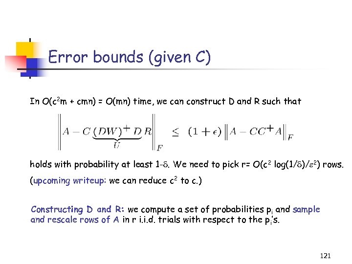Error bounds (given C) In O(c 2 m + cmn) = O(mn) time, we can construct D and R such that holds with probability at least 1 -. We need to pick r= O(c 2 log(1/ )/ 2) rows. (upcoming writeup: we can reduce c 2 to c. ) Constructing D and R: we compute a set of probabilities pi and sample and rescale rows of A in r i. i. d. trials with respect to the pi’s. 121

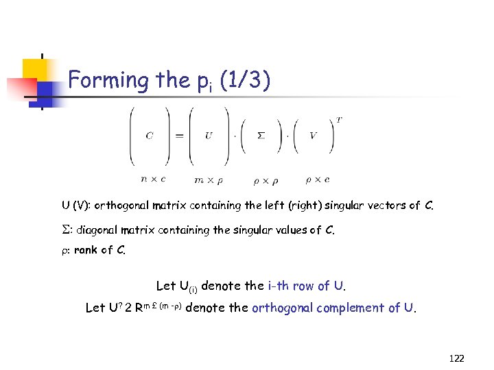Forming the pi (1/3) U (V): orthogonal matrix containing the left (right) singular vectors of C. : diagonal matrix containing the singular values of C. : rank of C. Let U(i) denote the i-th row of U. Let U? 2 Rm £ (m - ) denote the orthogonal complement of U. 122

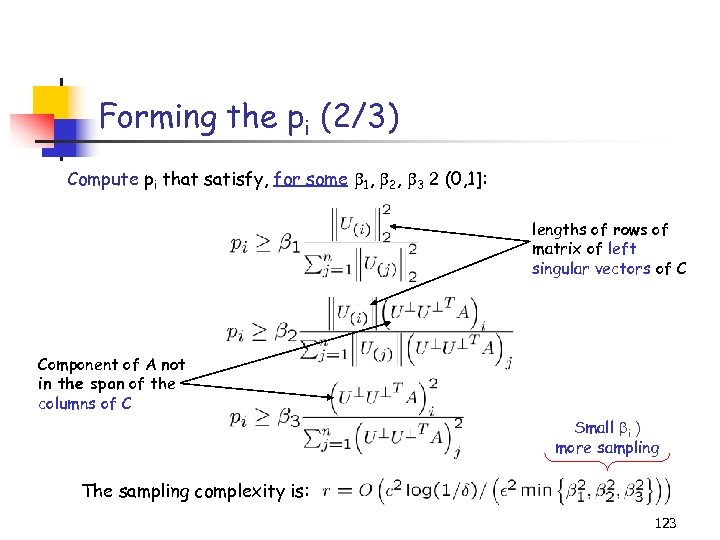Forming the pi (2/3) Compute pi that satisfy, for some 1, 2, 3 2 (0, 1]: lengths of rows of matrix of left singular vectors of C Component of A not in the span of the columns of C Small i ) more sampling The sampling complexity is: 123

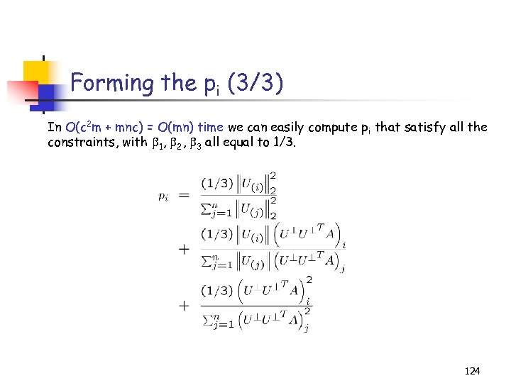Forming the pi (3/3) In O(c 2 m + mnc) = O(mn) time we can easily compute pi that satisfy all the constraints, with 1, 2, 3 all equal to 1/3. 124

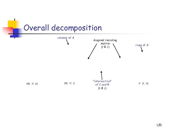Overall decomposition columns of A diagonal rescaling matrix (r £ c) rows of A ”intersection” of C and R (r £ c) 125

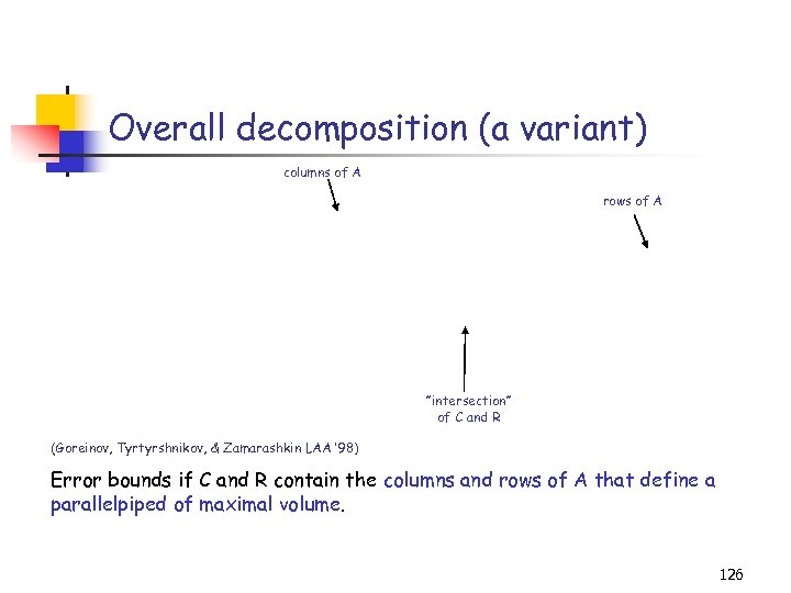Overall decomposition (a variant) columns of A rows of A ”intersection” of C and R (Goreinov, Tyrtyrshnikov, & Zamarashkin LAA ’ 98) Error bounds if C and R contain the columns and rows of A that define a parallelpiped of maximal volume. 126

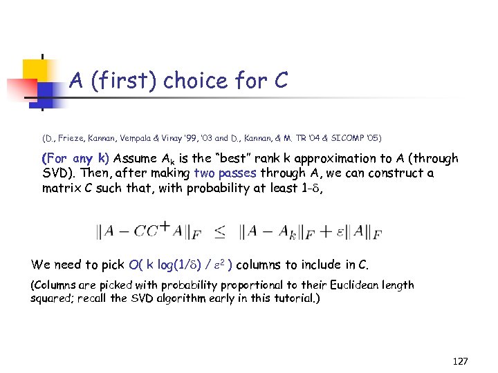A (first) choice for C (D. , Frieze, Kannan, Vempala & Vinay ’ 99, ‘ 03 and D. , Kannan, & M. TR ‘ 04 & SICOMP ‘ 05) (For any k) Assume Ak is the “best” rank k approximation to A (through SVD). Then, after making two passes through A, we can construct a matrix C such that, with probability at least 1 - , We need to pick O( k log(1/ ) / 2 ) columns to include in C. (Columns are picked with probability proportional to their Euclidean length squared; recall the SVD algorithm early in this tutorial. ) 127

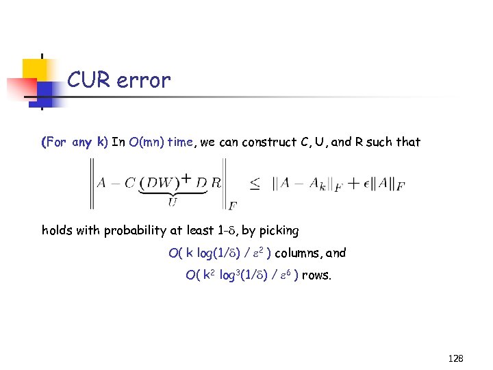CUR error (For any k) In O(mn) time, we can construct C, U, and R such that holds with probability at least 1 - , by picking O( k log(1/ ) / 2 ) columns, and O( k 2 log 3(1/ ) / 6 ) rows. 128

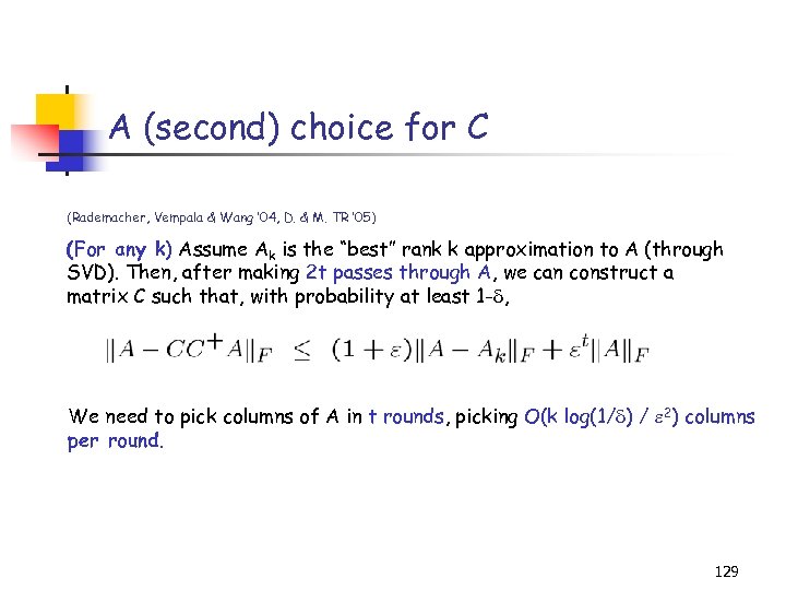A (second) choice for C (Rademacher, Vempala & Wang ’ 04, D. & M. TR ’ 05) (For any k) Assume Ak is the “best” rank k approximation to A (through SVD). Then, after making 2 t passes through A, we can construct a matrix C such that, with probability at least 1 - , We need to pick columns of A in t rounds, picking O(k log(1/ ) / 2) columns per round. 129

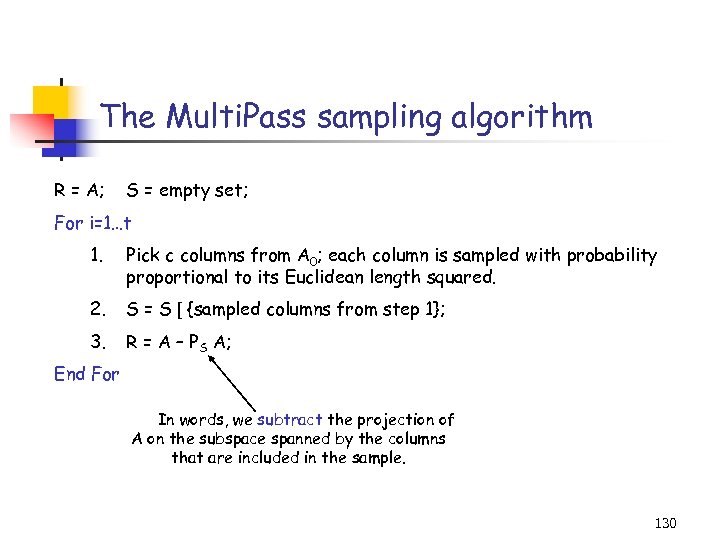The Multi. Pass sampling algorithm R = A; S = empty set; For i=1…t 1. Pick c columns from A 0; each column is sampled with probability proportional to its Euclidean length squared. 2. S = S [ {sampled columns from step 1}; 3. R = A – PS A; End For In words, we subtract the projection of A on the subspace spanned by the columns that are included in the sample. 130

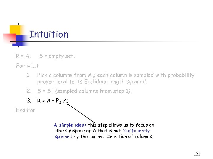Intuition R = A; S = empty set; For i=1…t 1. Pick c columns from A 0; each column is sampled with probability proportional to its Euclidean length squared. 2. S = S [ {sampled columns from step 1}; 3. R = A – PS A; End For A simple idea: this step allows us to focus on the subspace of A that is not “sufficiently” spanned by the current selection of columns. 131

CUR error (For any k) In O(mnt) time, we can construct C, U, and R such that holds with probability at least 1 - , by picking O( t k log(1/ ) / 2 ) columns, and O( t 2 k 2 log 3(1/ ) / 6 ) rows. 132

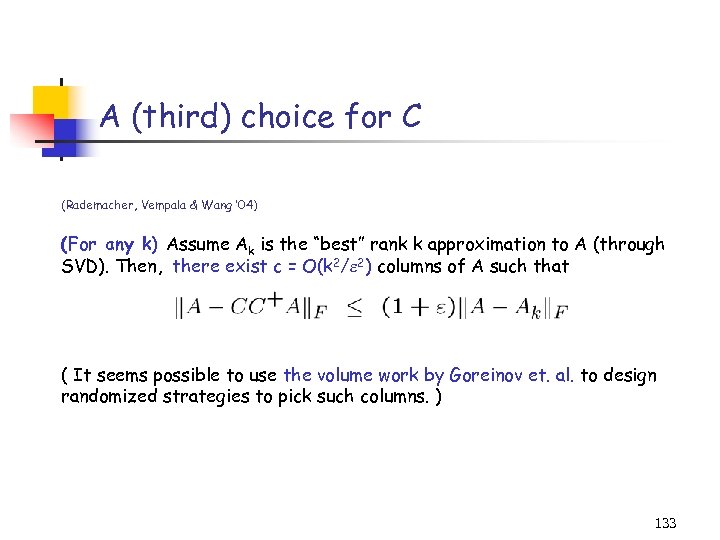A (third) choice for C (Rademacher, Vempala & Wang ’ 04) (For any k) Assume Ak is the “best” rank k approximation to A (through SVD). Then, there exist c = O(k 2/ 2) columns of A such that ( It seems possible to use the volume work by Goreinov et. al. to design randomized strategies to pick such columns. ) 133

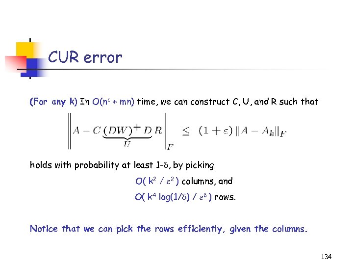CUR error (For any k) In O(nc + mn) time, we can construct C, U, and R such that holds with probability at least 1 - , by picking O( k 2 / 2 ) columns, and O( k 4 log(1/ ) / 6 ) rows. Notice that we can pick the rows efficiently, given the columns. 134

Example: finding ht-SNPs (data from K. Kidd’s lab at Yale University, joint work with Dr. Paschou at Yale University) Single Nucleotide Polymorphisms: the most common type of genetic variation in the genome. (Locations at the human genome where typically two alternate nucleotide bases are observed. ) Why are SNPs important: they occur quite frequently within the genome allowing the tracking of disease genes and population histories. Thus, they are effective markers for genomic research! There are ∼ 10 million SNPs in the human genome (under some assumptions). 135

Research topics Research Topics (working within a specific chromosomal region of the human genome) : (i) Are different SNPs correlated, either within a population, or across different populations? (Folklore knowledge: yes). (ii) Find a “good” set of haplotype tagging-SNPs capturing the diversity of a chromosomal region of the human genome. (iii) Is extrapolation feasible? (Recall Nystrom/CUR extrapolation. ) This would save (a lot of) time and money! Existing literature Pairwise metrics of SNP correlation, called LD (linkage disequilibrium) distance, based on nucleotide frequencies and co-occurrences. Almost no metrics exist for measuring correlation between more than 2 SNPs and LD is very difficult to generalize. Exhaustive and semi-exhaustive algorithms in order to pick “good” ht-SNPs that have small LD distance with all other SNPs. Using Linear Algebra: an SVD based algorithm was proposed by Lin & Altman, Am. J. Hum. Gen. 2004. 136

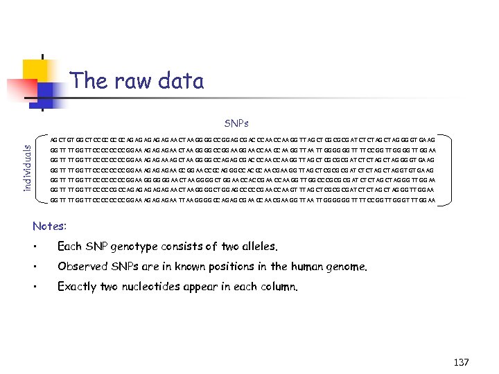The raw data SNPs individuals AG CT GT GG CT CC CC AG AG AG AA CT AA GG GG CC GG AG CG AC CC AA GG TT AG CT CG CG CG AT CT CT AG GG GT GA AG GG TT TT GG TT CC CC GG AA AG AG AG AA CT AA GG GG CC GG AA CC AA GG TT AA TT GG GG GG TT TT CC GG TT GG AA GG TT TT GG TT CC CC GG AA AG AG AA AG CT AA GG GG CC AG AG CG AC CC AA GG TT AG CT CG CG CG AT CT CT AG GG GT GA AG GG TT TT GG TT CC CC GG AA AG AG AG AA CC GG AA CC CC AG GG CC AC CC AA CG AA GG TT AG CT CG CG CG AT CT CT AG GT GT GA AG GG TT TT GG TT CC CC GG AA GG GG GG AA CT AA GG GG CT GG AA CC AC CG AA CC AA GG TT GG CC CG CG CG AT CT CT AG GG TT GG AA GG TT TT GG TT CC CC CG CC AG AG AG AA CT AA GG GG CT GG AG CC CC CG AA CC AA GT TT AG CT CG CG CG AT CT CT AG GG TT GG AA GG TT TT GG TT CC CC GG AA AG AG AG AA TT AA GG GG CC AG AG CG AA CC AA CG AA GG TT AA TT GG GG GG TT TT CC GG TT GG GT TT GG AA Notes: • Each SNP genotype consists of two alleles. • Observed SNPs are in known positions in the human genome. • Exactly two nucleotides appear in each column. 137

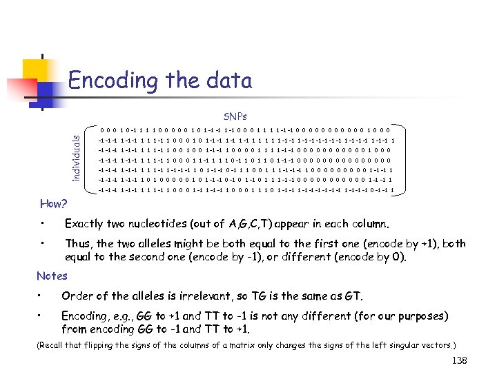Encoding the data SNPs individuals 0 0 0 1 0 -1 1 0 0 0 1 -1 -1 0 0 0 1 1 -1 -1 0 0 0 1 0 0 0 -1 -1 -1 1 1 1 -1 1 0 0 0 1 -1 -1 1 1 -1 -1 -1 1 -1 -1 1 -1 1 0 0 1 -1 -1 1 0 0 1 1 -1 -1 0 0 0 1 0 0 0 -1 -1 -1 1 1 1 -1 1 0 0 0 1 1 -1 1 0 1 -1 -1 0 0 0 0 -1 -1 -1 1 1 1 -1 -1 -1 1 0 1 -1 -1 0 -1 1 1 0 0 1 1 1 -1 -1 -1 1 0 0 0 0 0 1 -1 -1 -1 1 0 0 0 1 0 1 -1 -1 0 1 1 1 -1 -1 0 0 0 1 -1 -1 -1 1 -1 1 0 0 0 1 -1 -1 1 0 0 0 1 1 1 0 1 -1 -1 1 -1 -1 -1 0 -1 -1 1 How? • Exactly two nucleotides (out of A, G, C, T) appear in each column. • Thus, the two alleles might be both equal to the first one (encode by +1), both equal to the second one (encode by -1), or different (encode by 0). Notes • Order of the alleles is irrelevant, so TG is the same as GT. • Encoding, e. g. , GG to +1 and TT to -1 is not any different (for our purposes) from encoding GG to -1 and TT to +1. (Recall that flipping the signs of the columns of a matrix only changes the signs of the left singular vectors. ) 138

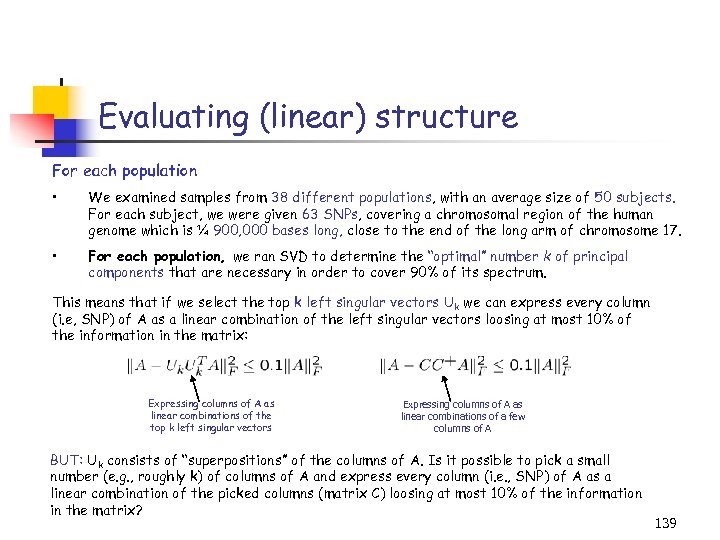Evaluating (linear) structure For each population • We examined samples from 38 different populations, with an average size of 50 subjects. For each subject, we were given 63 SNPs, covering a chromosomal region of the human genome which is ¼ 900, 000 bases long, close to the end of the long arm of chromosome 17. • For each population, we ran SVD to determine the “optimal” number k of principal components that are necessary in order to cover 90% of its spectrum. This means that if we select the top k left singular vectors Uk we can express every column (i. e, SNP) of A as a linear combination of the left singular vectors loosing at most 10% of the information in the matrix: Expressing columns of A as linear combinations of the top k left singular vectors Expressing columns of A as linear combinations of a few columns of A BUT: Uk consists of “superpositions” of the columns of A. Is it possible to pick a small number (e. g. , roughly k) of columns of A and express every column (i. e. , SNP) of A as a linear combination of the picked columns (matrix C) loosing at most 10% of the information in the matrix? 139

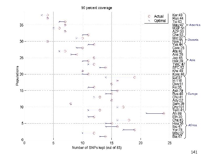
Algorithms • We ran various schemes to select “good” columns (i. e. , ht-SNPs). • A greedy Multi-Pass heuristic scheme gave the best results. (Select one column in each round, subtracting from A the projection of A on this column and repeating. ) Notice that some provable results exist for similar algorithms. Nice feature: SVD provides a non-trivial (maybe not achievable) lower bound. In many cases, the lower bound is attained by the greedy heuristic! (In our data, at most k+5 columns suffice to extract 90% of the structure. ) 140

America Oceania Asia Europe Africa 141

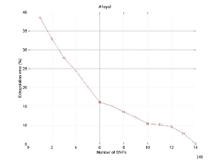
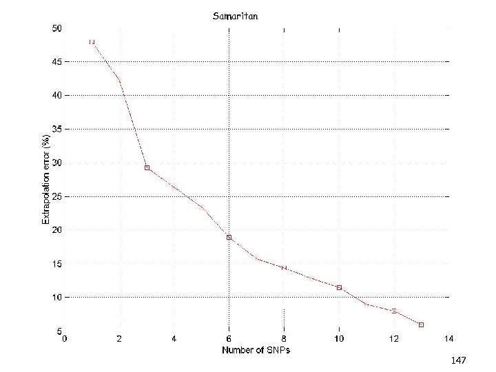
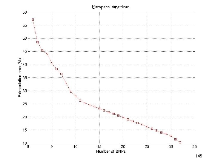
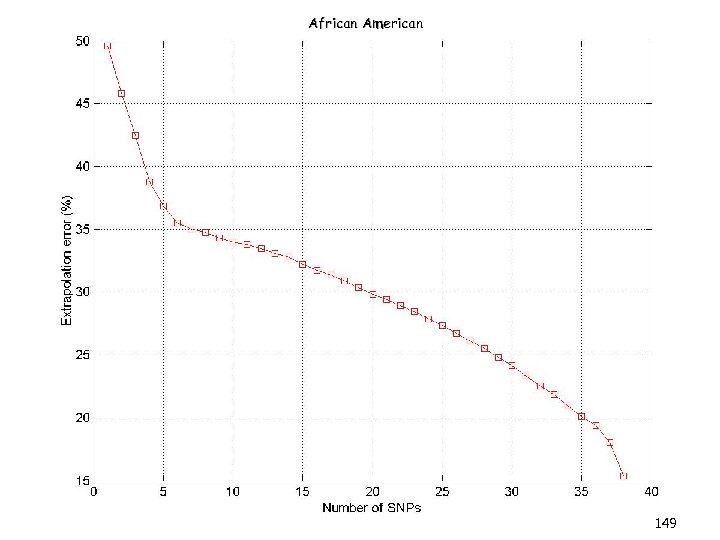
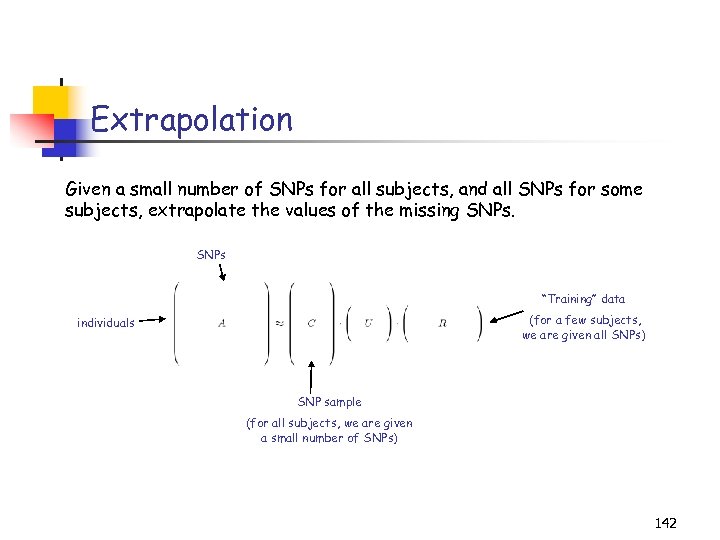Extrapolation Given a small number of SNPs for all subjects, and all SNPs for some subjects, extrapolate the values of the missing SNPs “Training” data (for a few subjects, we are given all SNPs) individuals SNP sample (for all subjects, we are given a small number of SNPs) 142

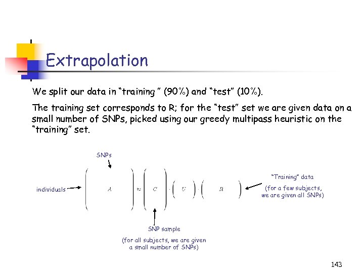Extrapolation We split our data in “training ” (90%) and “test” (10%). The training set corresponds to R; for the “test” set we are given data on a small number of SNPs, picked using our greedy multipass heuristic on the “training” set. SNPs “Training” data (for a few subjects, we are given all SNPs) individuals SNP sample (for all subjects, we are given a small number of SNPs) 143

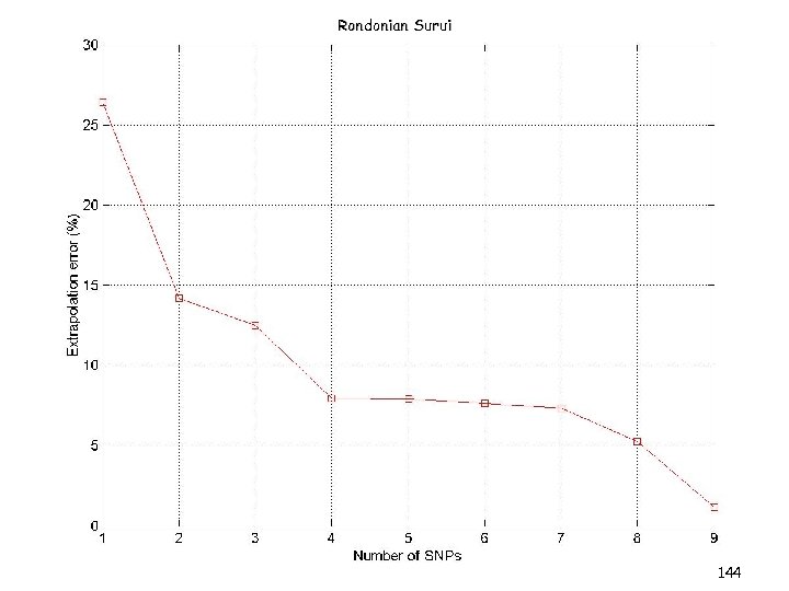Rondonian Surui 144

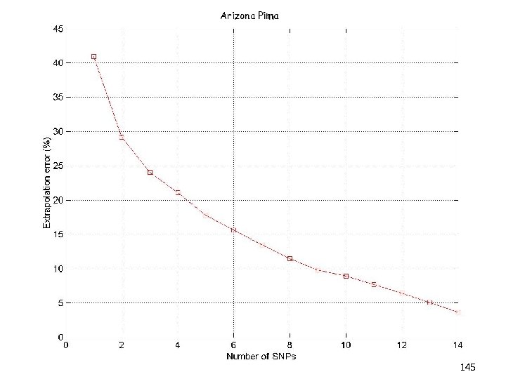Arizona Pima 145

Atayal 146

Samaritan 147

European American 148

African American 149

Conclusions & Open Problems • Empirical evaluation of different sampling probabilities • Uniform • Row/column lengths squared • Lengths of the rows of the left/right singular vectors • Inverse squares of row/column lengths to pick outliers • Others, depending on the problem to be solved? • Empirical evaluation for different learning problems Matrix reconstruction, regression, classification, clustering, etc. • Use CUR for improved interpretability for data matrices Structural vs. algorithmic issues • Use CW+CT for improved interpretability of Gram Matrices Structural vs. algorithmic issues 151

Conclusions & Open Problems • Impose other structural properties in CUR-type decompositions • Non-negativity • Element quantization, e. g. , to 0, 1, -1 • Block-SVD type structure • Robust heuristics and robust extensions Especially for noisy data • Quasi Monte-Carlo vs. Deterministic heuristics of the sketch for different data sets Especially for not-so-large datasets • Relate the pass-efficient framework to practice • passes over the data • a priori knowledge regarding data generation • oracle based models 152