db4932f388cd0b3f03dadc3c12e319f4.ppt
- Количество слайдов: 164
Tutorial on Bayesian Networks Jack Breese Daphne Koller Microsoft Research Stanford University breese@microsoft. com koller@cs. stanford. edu First given as a AAAI’ 97 tutorial. 1
Overview n Decision-theoretic techniques u Explicit management of uncertainty and tradeoffs u Probability theory u Maximization of expected utility n Applications to AI problems u Diagnosis u Expert systems u Planning u Learning © Jack Breese (Microsoft) & Daphne Koller (Stanford) 2
Science- AAAI-97 n Model Minimization in Markov Decision Processes n Effective Bayesian Inference for Stochastic Programs n Learning Bayesian Networks from Incomplete Data n Summarizing CSP Hardness With Continuous Probability Distributions n Speeding Safely: Multi-criteria Optimization in Probabilistic Planning n Structured Solution Methods for Non-Markovian Decision Processes © Jack Breese (Microsoft) & Daphne Koller (Stanford) 3

Applications Microsoft's cost-cutting helps users 04/21/97 A Microsoft Corp. strategy to cut its support costs by letting users solve their own problems using electronic means is paying off for users. In March, the company began rolling out a series of Troubleshooting Wizards on its World Wide Web site. Troubleshooting Wizards save time and money for users who don't have Windows NT specialists on hand at all times, said Paul Soares, vice president and general manager of Alden Buick Pontiac, a General Motors Corp. car dealership in Fairhaven, Mass © Jack Breese (Microsoft) & Daphne Koller (Stanford) 4
Course Contents » Concepts in Probability u Random variables u Basic properties (Bayes rule) Bayesian Networks n Inference n Decision making n Learning networks from data n Reasoning over time n Applications n © Jack Breese (Microsoft) & Daphne Koller (Stanford) 6
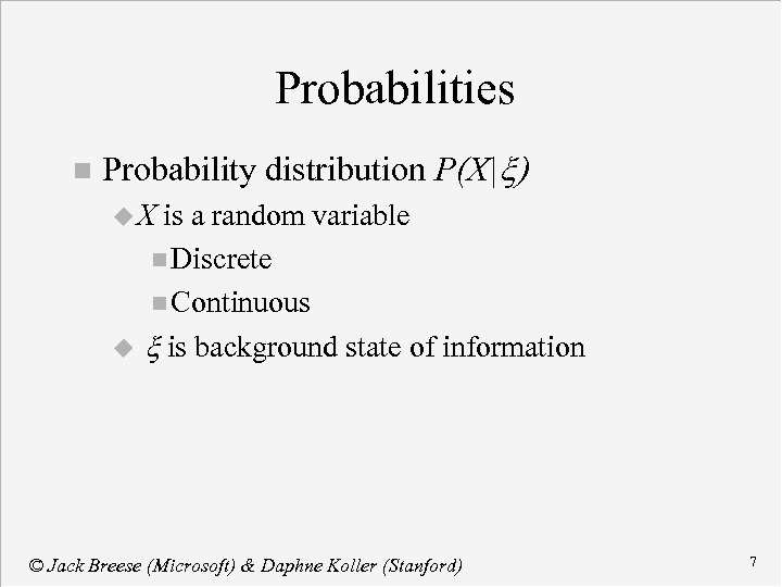
Probabilities n Probability distribution P(X|x) u. X is a random variable n Discrete n Continuous u x is background state of information © Jack Breese (Microsoft) & Daphne Koller (Stanford) 7
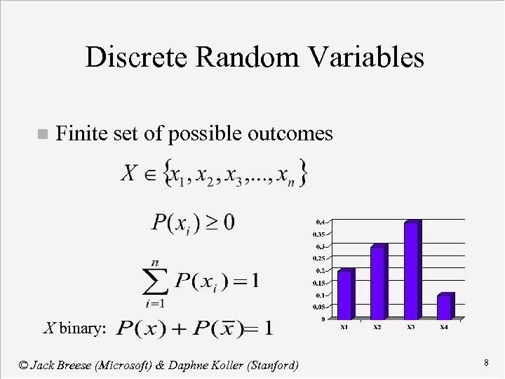
Discrete Random Variables n Finite set of possible outcomes X binary: © Jack Breese (Microsoft) & Daphne Koller (Stanford) 8
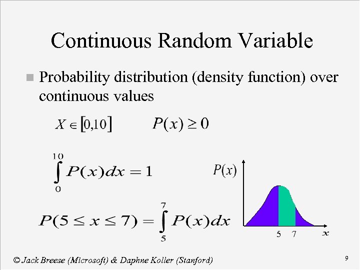
Continuous Random Variable n Probability distribution (density function) over continuous values 5 © Jack Breese (Microsoft) & Daphne Koller (Stanford) 7 9
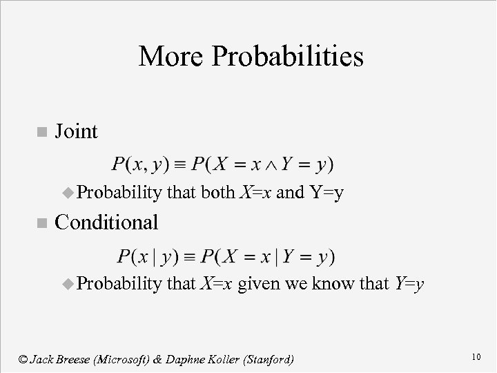
More Probabilities n Joint u Probability n that both X=x and Y=y Conditional u Probability that X=x given we know that Y=y © Jack Breese (Microsoft) & Daphne Koller (Stanford) 10
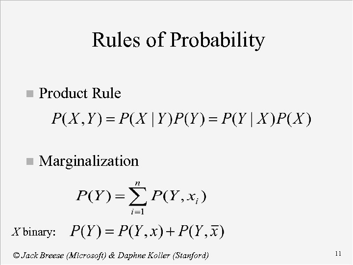
Rules of Probability n Product Rule n Marginalization X binary: © Jack Breese (Microsoft) & Daphne Koller (Stanford) 11
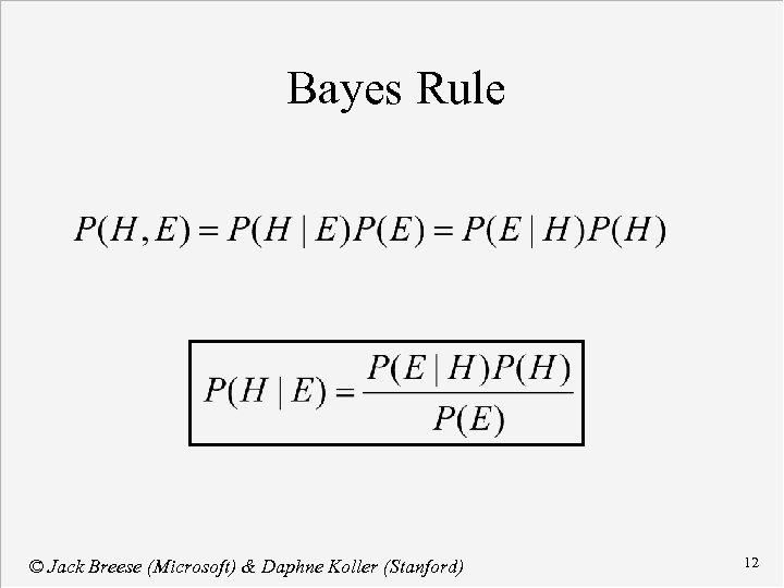
Bayes Rule © Jack Breese (Microsoft) & Daphne Koller (Stanford) 12
Course Contents n » Concepts in Probability Bayesian Networks u Basics u Additional structure u Knowledge acquisition Inference n Decision making n Learning networks from data n Reasoning over time n Applications n © Jack Breese (Microsoft) & Daphne Koller (Stanford) 13
Bayesian networks n Basics u Structured representation u Conditional independence u Naïve Bayes model u Independence facts © Jack Breese (Microsoft) & Daphne Koller (Stanford) 14
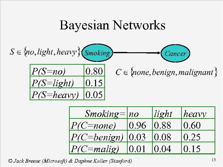
Bayesian Networks Smoking Cancer P(S=no) 0. 80 P(S=light) 0. 15 P(S=heavy) 0. 05 Smoking= P(C=none) P(C=benign) P(C=malig) no 0. 96 0. 03 0. 01 © Jack Breese (Microsoft) & Daphne Koller (Stanford) light 0. 88 0. 04 heavy 0. 60 0. 25 0. 15 15
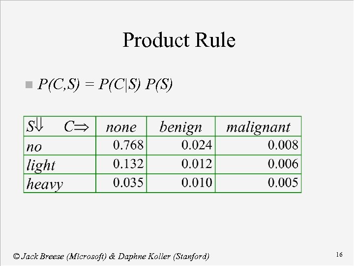
Product Rule n P(C, S) = P(C|S) P(S) © Jack Breese (Microsoft) & Daphne Koller (Stanford) 16

Marginalization P(Smoke) P(Cancer) © Jack Breese (Microsoft) & Daphne Koller (Stanford) 17
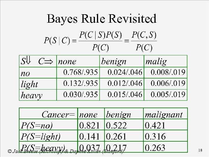
Bayes Rule Revisited Cancer= none benign P(S=no) 0. 821 0. 522 P(S=light) 0. 141 0. 261 P(S=heavy) 0. 037 0. 217 © Jack Breese (Microsoft) & Daphne Koller (Stanford) malignant 0. 421 0. 316 0. 263 18
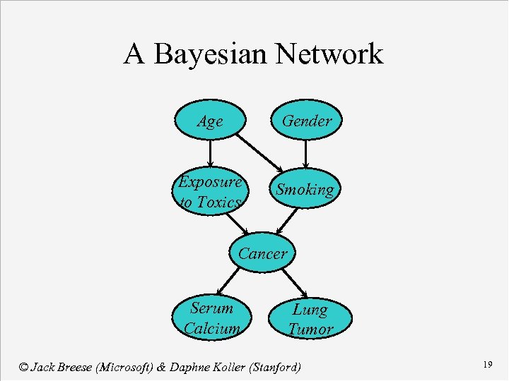
A Bayesian Network Age Gender Exposure to Toxics Smoking Cancer Serum Calcium Lung Tumor © Jack Breese (Microsoft) & Daphne Koller (Stanford) 19
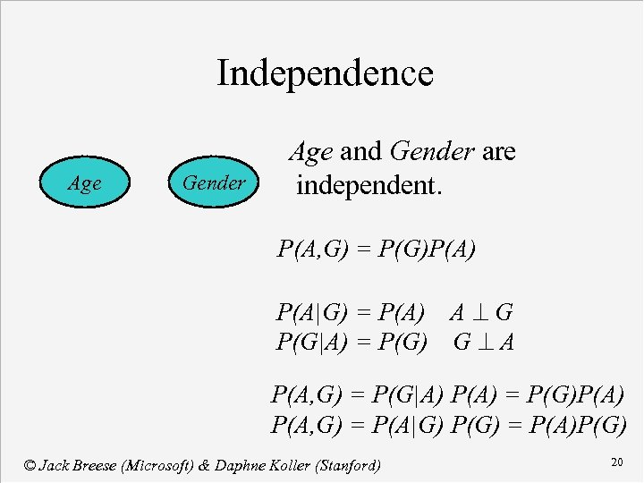
Independence Age Gender Age and Gender are independent. P(A, G) = P(G)P(A) P(A|G) = P(A) A ^ G P(G|A) = P(G) G ^ A P(A, G) = P(G|A) P(A) = P(G)P(A) P(A, G) = P(A|G) P(G) = P(A)P(G) © Jack Breese (Microsoft) & Daphne Koller (Stanford) 20
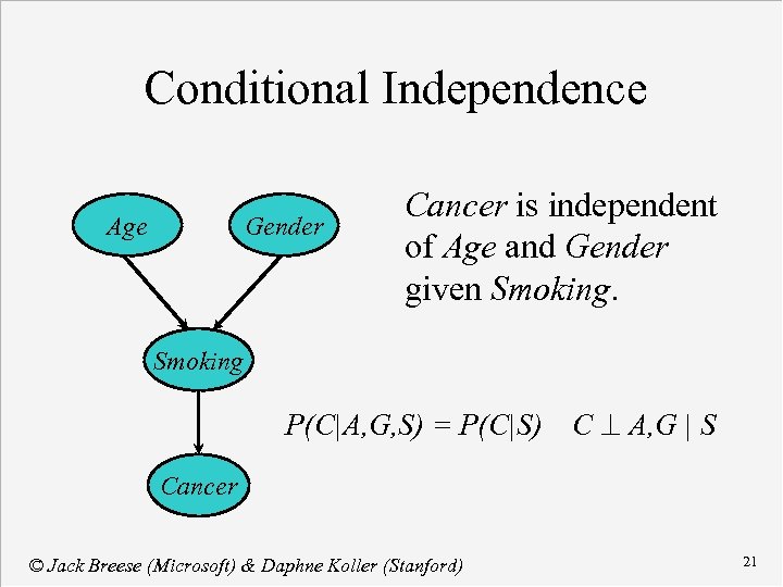
Conditional Independence Age Gender Cancer is independent of Age and Gender given Smoking P(C|A, G, S) = P(C|S) C ^ A, G | S Cancer © Jack Breese (Microsoft) & Daphne Koller (Stanford) 21
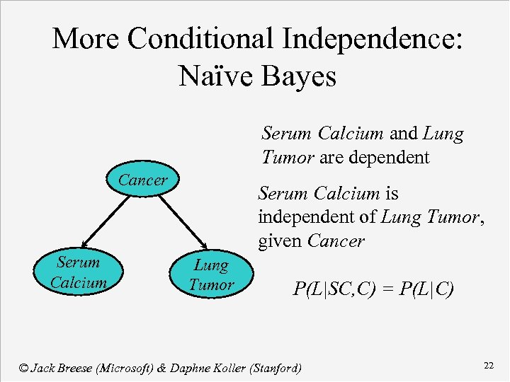
More Conditional Independence: Naïve Bayes Serum Calcium and Lung Tumor are dependent Cancer Serum Calcium is independent of Lung Tumor, given Cancer Lung Tumor P(L|SC, C) = P(L|C) © Jack Breese (Microsoft) & Daphne Koller (Stanford) 22
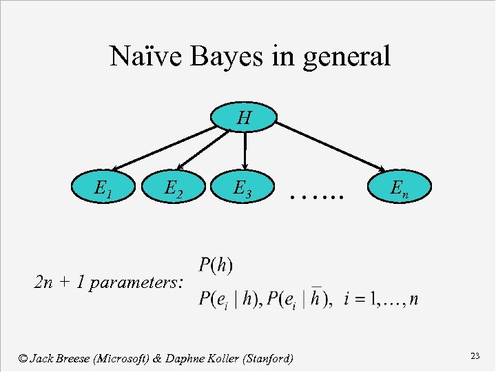
Naïve Bayes in general H E 1 E 2 E 3 …. . . En 2 n + 1 parameters: © Jack Breese (Microsoft) & Daphne Koller (Stanford) 23
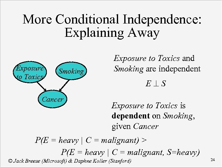
More Conditional Independence: Explaining Away Exposure to Toxics Smoking Cancer Exposure to Toxics and Smoking are independent E^S Exposure to Toxics is dependent on Smoking, given Cancer P(E = heavy | C = malignant) > P(E = heavy | C = malignant, S=heavy) © Jack Breese (Microsoft) & Daphne Koller (Stanford) 24
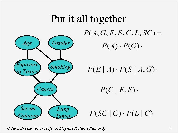
Put it all together Age Gender Exposure to Toxics Smoking Cancer Serum Calcium Lung Tumor © Jack Breese (Microsoft) & Daphne Koller (Stanford) 25
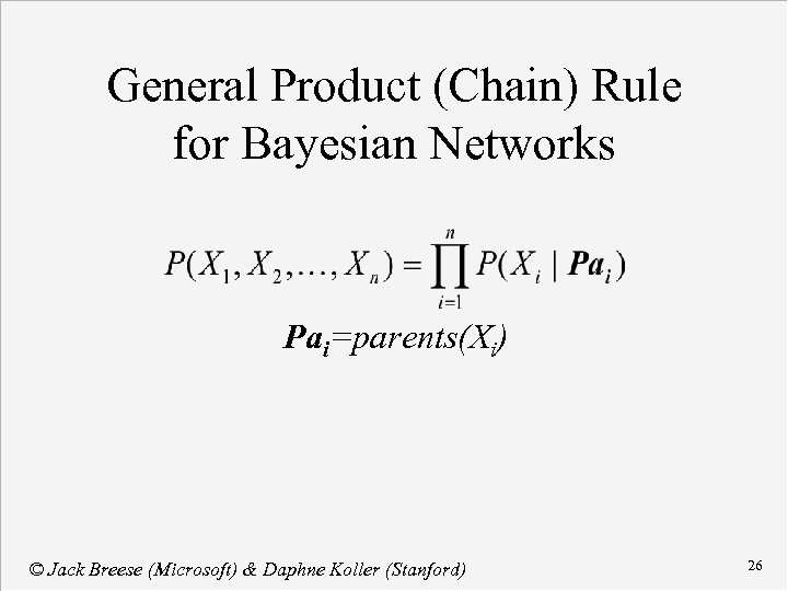
General Product (Chain) Rule for Bayesian Networks Pai=parents(Xi) © Jack Breese (Microsoft) & Daphne Koller (Stanford) 26
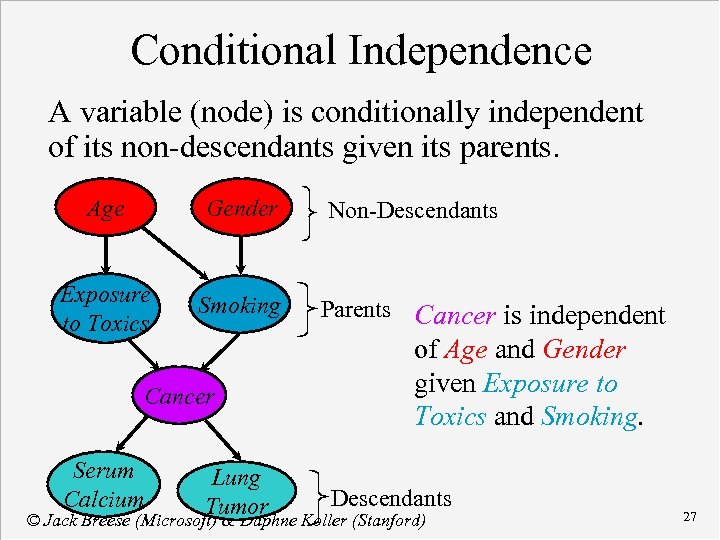
Conditional Independence A variable (node) is conditionally independent of its non-descendants given its parents. Age Gender Exposure to Toxics Smoking Cancer Serum Calcium Lung Tumor Non-Descendants Parents Cancer is independent of Age and Gender given Exposure to Toxics and Smoking. Descendants © Jack Breese (Microsoft) & Daphne Koller (Stanford) 27
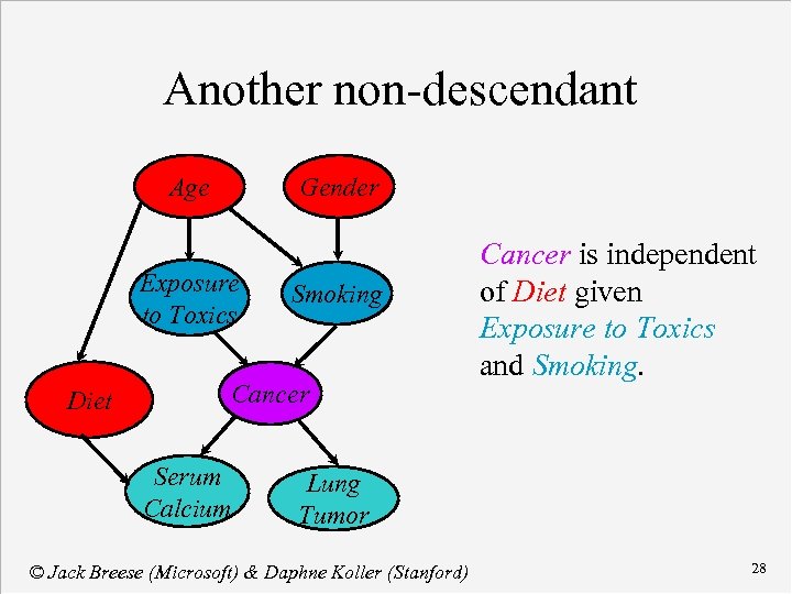
Another non-descendant Age Gender Exposure to Toxics Diet Smoking Cancer Serum Calcium Cancer is independent of Diet given Exposure to Toxics and Smoking. Lung Tumor © Jack Breese (Microsoft) & Daphne Koller (Stanford) 28
Independence and Graph Separation Given a set of observations, is one set of variables dependent on another set? n Observing effects can induce dependencies. n d-separation (Pearl 1988) allows us to check conditional independence graphically. n © Jack Breese (Microsoft) & Daphne Koller (Stanford) 29
Bayesian networks n Additional structure u Nodes as functions u Causal independence u Context specific dependencies u Continuous variables u Hierarchy and model construction © Jack Breese (Microsoft) & Daphne Koller (Stanford) 30
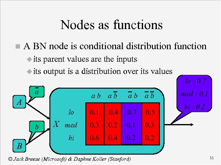
Nodes as functions n A BN node is conditional distribution function u its parent values are the inputs u its output is a distribution over its values lo : 0. 7 a ab ab A lo b B X med X hi ab ab 0. 1 0. 4 0. 7 0. 5 0. 3 0. 2 0. 1 0. 4 0. 2 hi : 0. 2 0. 3 0. 6 med : 0. 1 0. 2 © Jack Breese (Microsoft) & Daphne Koller (Stanford) 31
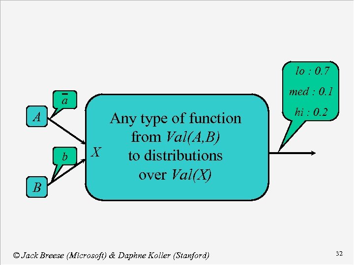
lo : 0. 7 med : 0. 1 a A b B Any type of function from Val(A, B) X X to distributions over Val(X) © Jack Breese (Microsoft) & Daphne Koller (Stanford) hi : 0. 2 32
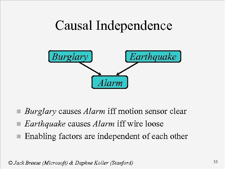
Causal Independence Burglary Earthquake Alarm n n n Burglary causes Alarm iff motion sensor clear Earthquake causes Alarm iff wire loose Enabling factors are independent of each other © Jack Breese (Microsoft) & Daphne Koller (Stanford) 33
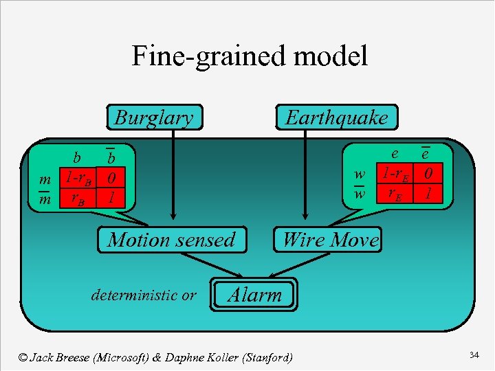
Fine-grained model Burglary Earthquake e e w 1 -r. E 0 w r. E 1 b b m 1 -r. B 0 m r. B 1 Motion sensed deterministic or Wire Move Alarm © Jack Breese (Microsoft) & Daphne Koller (Stanford) 34
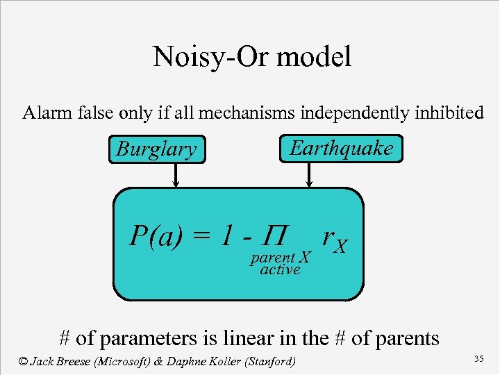
Noisy-Or model Alarm false only if all mechanisms independently inhibited Earthquake Burglary P(a) = 1 - parent X active r. X # of parameters is linear in the # of parents © Jack Breese (Microsoft) & Daphne Koller (Stanford) 35

CPCS Network © Jack Breese (Microsoft) & Daphne Koller (Stanford) 36
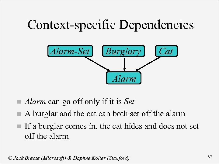
Context-specific Dependencies Alarm-Set Burglary Cat Alarm n n n Alarm can go off only if it is Set A burglar and the cat can both set off the alarm If a burglar comes in, the cat hides and does not set off the alarm © Jack Breese (Microsoft) & Daphne Koller (Stanford) 37
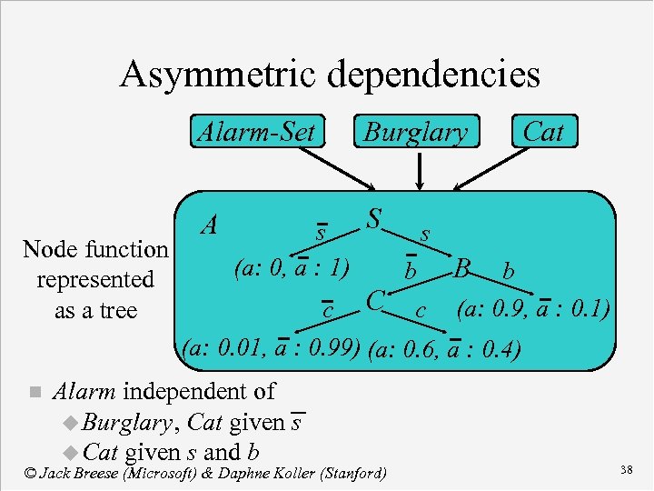
Asymmetric dependencies Alarm-Set Burglary Cat S s s Node function (a: 0, a : 1) b B b represented c C c (a: 0. 9, a : 0. 1) as a tree (a: 0. 01, a : 0. 99) (a: 0. 6, a : 0. 4) A n Alarm independent of u Burglary, Cat given s u Cat given s and b © Jack Breese (Microsoft) & Daphne Koller (Stanford) 38
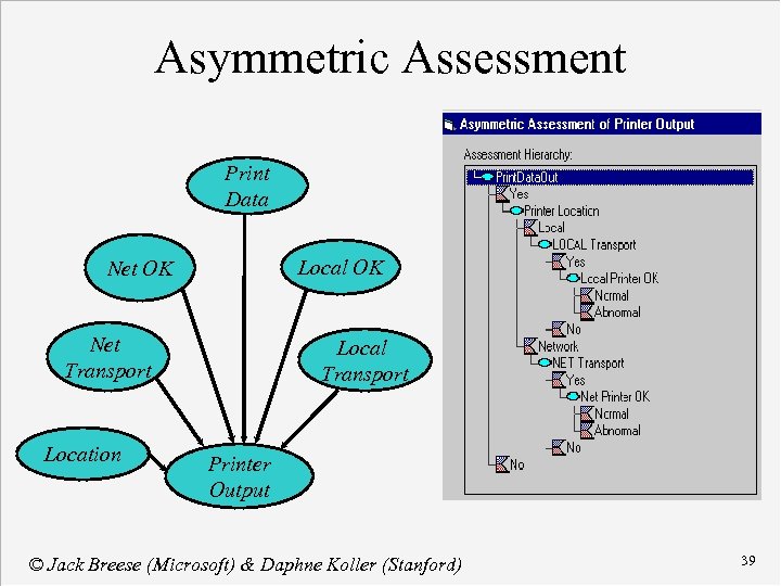
Asymmetric Assessment Print Data Local OK Net Transport Location Local Transport Printer Output © Jack Breese (Microsoft) & Daphne Koller (Stanford) 39
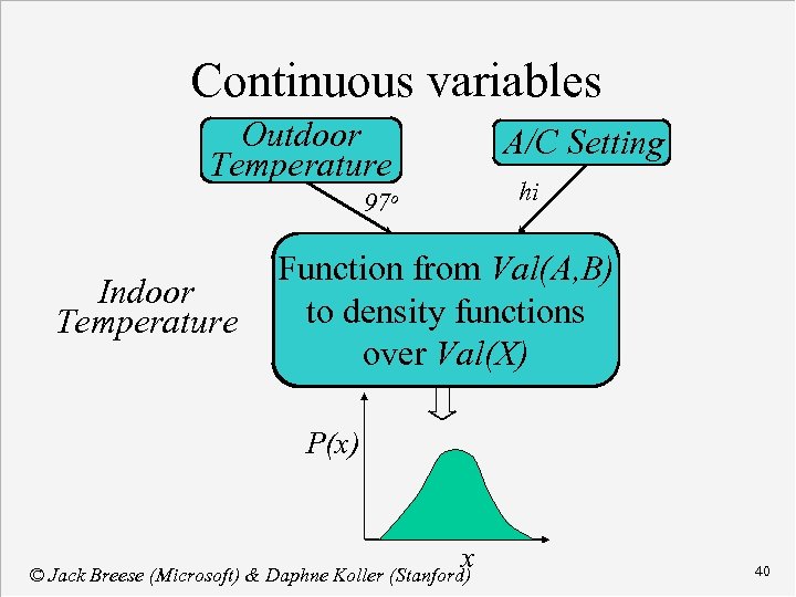
Continuous variables Outdoor Temperature A/C Setting hi 97 o Indoor Temperature Function from Val(A, B) Indoor to density functions Temperature over Val(X) P(x) x © Jack Breese (Microsoft) & Daphne Koller (Stanford) 40
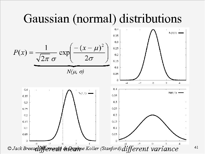
Gaussian (normal) distributions N(m, s) © Jack Breese (Microsoft) & Daphne Koller (Stanford) different mean variance 41
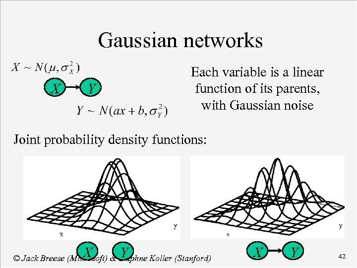
Gaussian networks X Y Each variable is a linear function of its parents, with Gaussian noise Joint probability density functions: X Y © Jack Breese (Microsoft) & Daphne Koller (Stanford) X Y 42
Composing functions Recall: a BN node is a function n We can compose functions to get more complex functions. n The result: A hierarchically structured BN. n Since functions can be called more than once, we can reuse a BN model fragment in multiple contexts. n © Jack Breese (Microsoft) & Daphne Koller (Stanford) 43
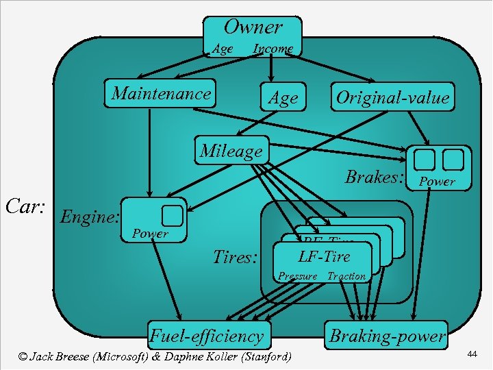
Owner Age Income Maintenance Age Original-value Mileage Brakes: Brakes Power Car: Engine Power RF-Tires LF-Tires: Pressure Traction Fuel-efficiency © Jack Breese (Microsoft) & Daphne Koller (Stanford) Braking-power 44
Bayesian Networks n Knowledge acquisition u Variables u Structure u Numbers © Jack Breese (Microsoft) & Daphne Koller (Stanford) 45
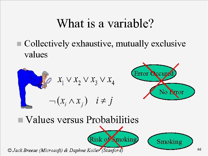
What is a variable? n Collectively exhaustive, mutually exclusive values Error Occured No Error n Values versus Probabilities Risk of Smoking © Jack Breese (Microsoft) & Daphne Koller (Stanford) Smoking 46
Clarity Test: Knowable in Principle Weather {Sunny, Cloudy, Rain, Snow} n Gasoline: Cents per gallon n Temperature { 100 F , < 100 F} n User needs help on Excel Charting {Yes, No} n User’s personality {dominant, submissive} n © Jack Breese (Microsoft) & Daphne Koller (Stanford) 47
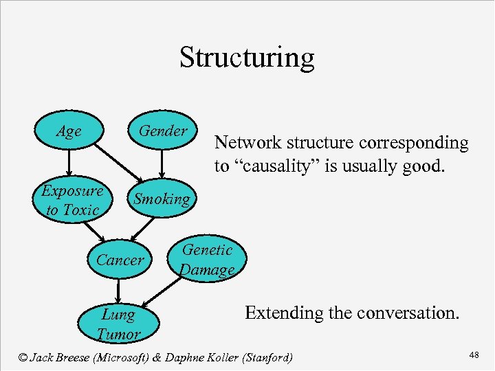
Structuring Age Gender Exposure to Toxic Smoking Cancer Lung Tumor Network structure corresponding to “causality” is usually good. Genetic Damage Extending the conversation. © Jack Breese (Microsoft) & Daphne Koller (Stanford) 48
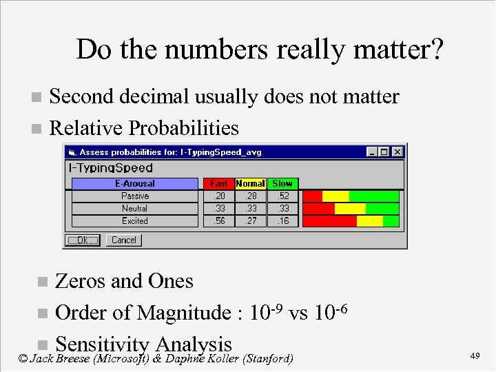
Do the numbers really matter? Second decimal usually does not matter n Relative Probabilities n Zeros and Ones n Order of Magnitude : 10 -9 vs 10 -6 n Sensitivity Analysis © Jack Breese (Microsoft) & Daphne Koller (Stanford) n 49
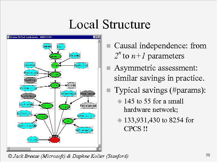
Local Structure n n n Causal independence: from 2 n to n+1 parameters Asymmetric assessment: similar savings in practice. Typical savings (#params): u 145 to 55 for a small hardware network; u 133, 931, 430 to 8254 for CPCS !! © Jack Breese (Microsoft) & Daphne Koller (Stanford) 50
Course Contents Concepts in Probability n Bayesian Networks » Inference n Decision making n Learning networks from data n Reasoning over time n Applications n © Jack Breese (Microsoft) & Daphne Koller (Stanford) 51
Inference Patterns of reasoning n Basic inference n Exact inference n Exploiting structure n Approximate inference n © Jack Breese (Microsoft) & Daphne Koller (Stanford) 52
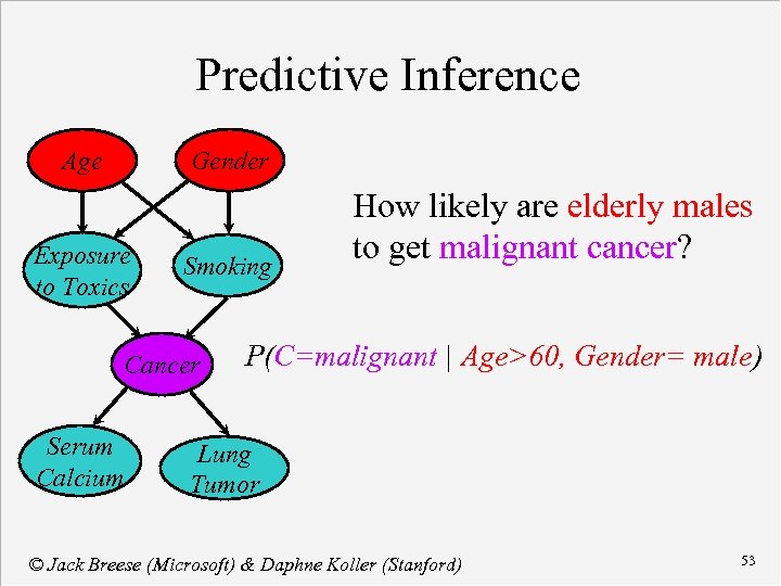
Predictive Inference Age Gender Exposure to Toxics Smoking Cancer Serum Calcium How likely are elderly males to get malignant cancer? P(C=malignant | Age>60, Gender= male) Lung Tumor © Jack Breese (Microsoft) & Daphne Koller (Stanford) 53
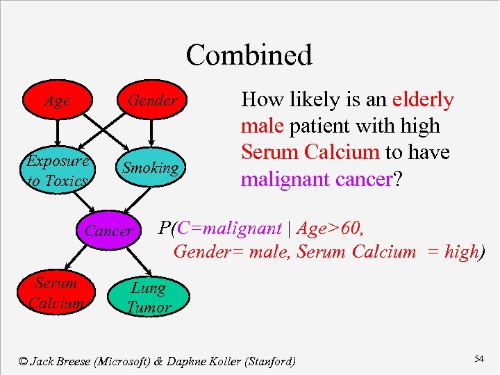
Combined Age Gender Exposure to Toxics Smoking Cancer Serum Calcium How likely is an elderly male patient with high Serum Calcium to have malignant cancer? P(C=malignant | Age>60, Gender= male, Serum Calcium = high) Lung Tumor © Jack Breese (Microsoft) & Daphne Koller (Stanford) 54
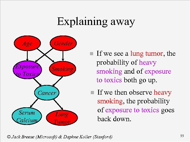
Explaining away Age Gender n Exposure to Toxics n If we then observe heavy smoking, the probability of exposure to toxics goes back down. Smoking Cancer Serum Calcium If we see a lung tumor, the probability of heavy smoking and of exposure to toxics both go up. Lung Tumor © Jack Breese (Microsoft) & Daphne Koller (Stanford) 55
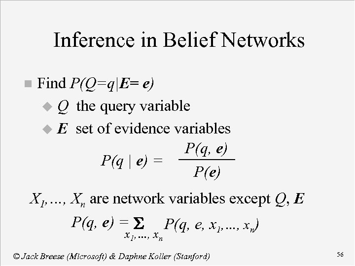
Inference in Belief Networks n Find P(Q=q|E= e) u Q the query variable u E set of evidence variables P(q, e) P(q | e) = P(e) X 1, …, Xn are network variables except Q, E P(q, e) = S P(q, e, x 1, …, xn) x 1, …, xn © Jack Breese (Microsoft) & Daphne Koller (Stanford) 56
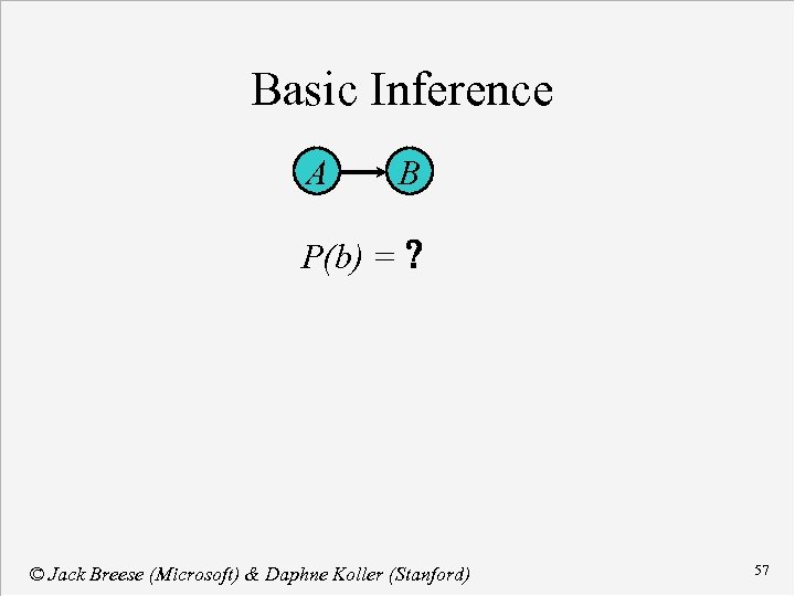
Basic Inference A B P(b) = ? © Jack Breese (Microsoft) & Daphne Koller (Stanford) 57
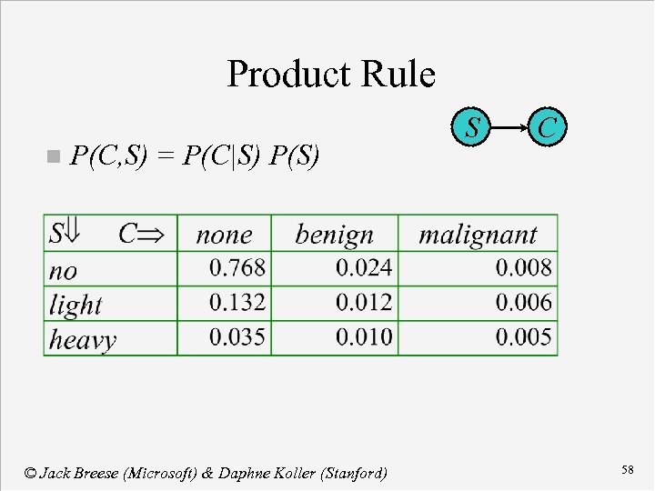
Product Rule n P(C, S) = P(C|S) P(S) © Jack Breese (Microsoft) & Daphne Koller (Stanford) S C 58
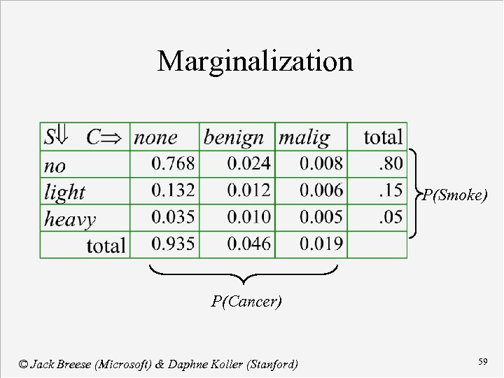
Marginalization P(Smoke) P(Cancer) © Jack Breese (Microsoft) & Daphne Koller (Stanford) 59
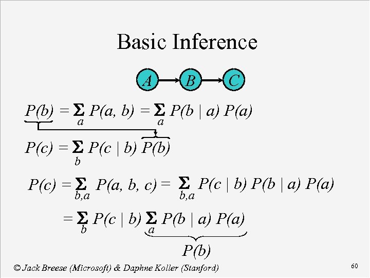
Basic Inference A B C P(b) = S P(a, b) = S P(b | a) P(a) a a P(c) = S P(c | b) P(b) b P(c) = S P(a, b, c) = S P(c | b) P(b | a) P(a) b, a = S P(c | b) S P(b | a) P(a) b a P(b) © Jack Breese (Microsoft) & Daphne Koller (Stanford) 60
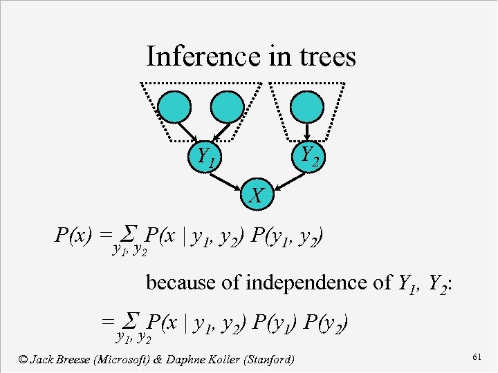
Inference in trees Y 2 Y 1 X P(x) =y. S y P(x | y 1, y 2) P(y 1, y 2) , 1 2 because of independence of Y 1, Y 2: = S P(x | y 1, y 2) P(y 1) P(y 2) y 1, y 2 © Jack Breese (Microsoft) & Daphne Koller (Stanford) 61
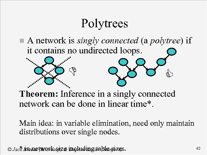
Polytrees n A network is singly connected (a polytree) if it contains no undirected loops. D C Theorem: Inference in a singly connected network can be done in linear time*. Main idea: in variable elimination, need only maintain distributions over single nodes. * in network size Daphne Koller (Stanford) © Jack Breese (Microsoft) & including table sizes. 62
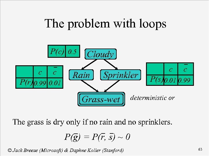
The problem with loops P(c) 0. 5 c c P(r) 0. 99 0. 01 Cloudy Rain Sprinkler Grass-wet c c P(s) 0. 01 0. 99 deterministic or The grass is dry only if no rain and no sprinklers. P(g) = P(r, s) ~ 0 © Jack Breese (Microsoft) & Daphne Koller (Stanford) 63
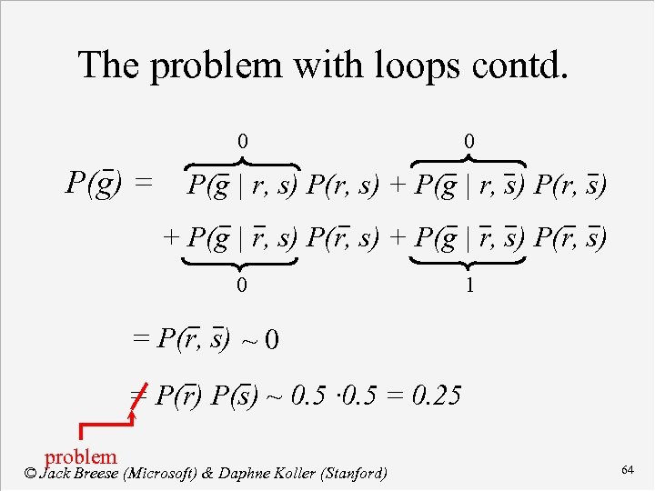
The problem with loops contd. 0 P(g) = 0 P(g | r, s) P(r, s) + P(g | r, s) P(r, s) 0 1 = P(r, s) ~ 0 = P(r) P(s) ~ 0. 5 · 0. 5 = 0. 25 problem © Jack Breese (Microsoft) & Daphne Koller (Stanford) 64
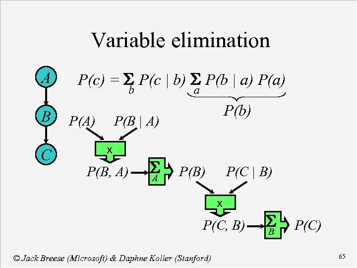
Variable elimination A B C P(c) = S P(c | b) S P(b | a) P(a) b P(A) a P(b) P(B | A) x P(B, A) S A P(B) P(C | B) x P(C, B) © Jack Breese (Microsoft) & Daphne Koller (Stanford) S B P(C) 65
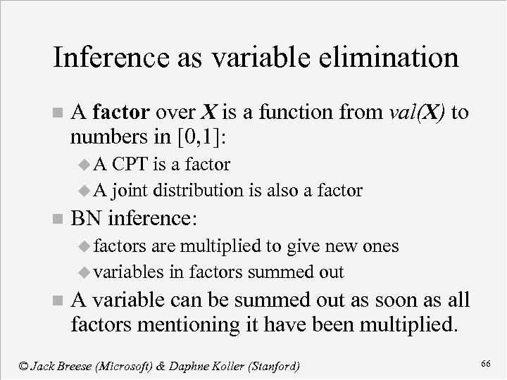
Inference as variable elimination n A factor over X is a function from val(X) to numbers in [0, 1]: u. A CPT is a factor u A joint distribution is also a factor n BN inference: u factors are multiplied to give new ones u variables in factors summed out n A variable can be summed out as soon as all factors mentioning it have been multiplied. © Jack Breese (Microsoft) & Daphne Koller (Stanford) 66
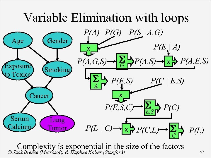
Variable Elimination with loops Age Gender Exposure to Toxics Smoking P(A) P(G) P(S | A, G) P(E | A) x S G P(A, G, S) S A P(E, S) x Cancer P(E, S, C) Serum Calcium Lung Tumor P(L | C) x P(A, S) P(A, E, S) x P(C | E, S) S E, S P(C) P(C, L) S C Complexity is exponential in the size of the factors © Jack Breese (Microsoft) & Daphne Koller (Stanford) P(L) 67
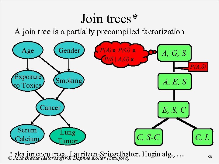
Join trees* A join tree is a partially precompiled factorization Age Gender P(A) x P(G) x P(S | A, G) x A, G, S P(A, S) Exposure to Toxics Smoking A, E, S Cancer Serum Calcium Lung Tumor E, S, C C, S-C * aka junction trees, Lauritzen-Spiegelhalter, Hugin alg. , … © Jack Breese (Microsoft) & Daphne Koller (Stanford) C, L 68
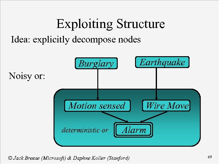
Exploiting Structure Idea: explicitly decompose nodes Earthquake Burglary Noisy or: Motion sensed deterministic or Wire Move Alarm © Jack Breese (Microsoft) & Daphne Koller (Stanford) 69
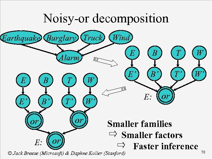
Noisy-or decomposition Earthquake Burglary Truck Wind E E B E’ T B’ T’ or W B’ T’ W’ E: W’ or or E: W T E’ Alarm B or Smaller families Smaller factors Faster inference © Jack Breese (Microsoft) & Daphne Koller (Stanford) 70
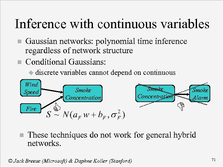
Inference with continuous variables Gaussian networks: polynomial time inference regardless of network structure Conditional Gaussians: n n u discrete variables cannot depend on continuous Wind Speed Fire n C Smoke Concentration D Smoke Alarm These techniques do not work for general hybrid networks. © Jack Breese (Microsoft) & Daphne Koller (Stanford) 71
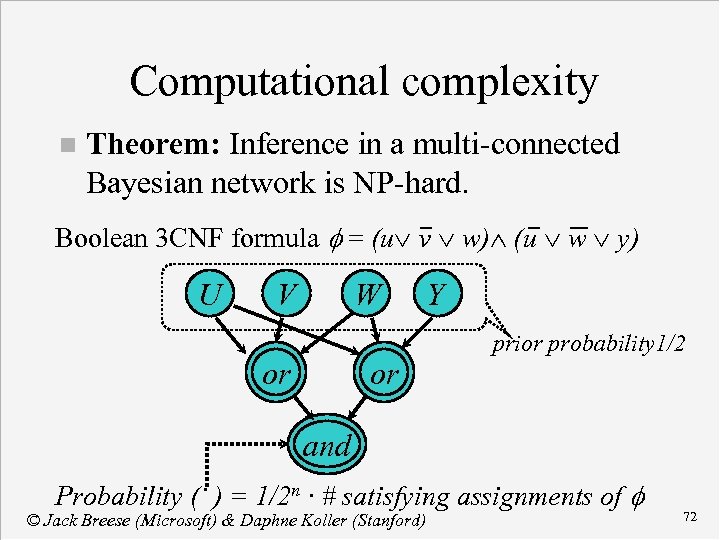
Computational complexity n Theorem: Inference in a multi-connected Bayesian network is NP-hard. Boolean 3 CNF formula f = (u v w) (u w y) U V W or or Y prior probability 1/2 and Probability ( ) = 1/2 n · # satisfying assignments of f © Jack Breese (Microsoft) & Daphne Koller (Stanford) 72
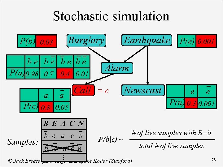
Stochastic simulation Burglary P(b) 0. 03 be be P(a) 0. 98 0. 7 0. 4 0. 01 a a Earthquake P(e) 0. 001 Alarm Call = c Newscast e e P(n) 0. 3 0. 001 P(c) 0. 8 0. 05 B E A C N Samples: b e a c n P(b|c) ~ # of live samples with B=b b e a c n . . . © Jack Breese (Microsoft) & Daphne Koller (Stanford) total # of live samples 73
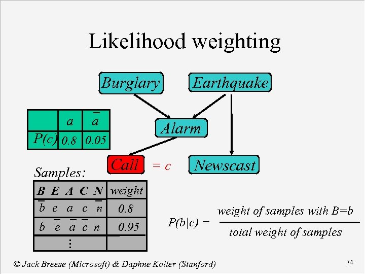
Likelihood weighting Burglary a a Alarm P(c) 0. 8 0. 05 Samples: Earthquake Call = c B E A C N weight b e a c n 0. 8 b e a c n 0. 95 Newscast P(b|c) = weight of samples with B=b total weight of samples . . . © Jack Breese (Microsoft) & Daphne Koller (Stanford) 74
Other approaches n Search based techniques u search for high-probability instantiations u use instantiations to approximate probabilities n Structural approximation u simplify network n eliminate edges, nodes n abstract node values n simplify CPTs u do inference in simplified network © Jack Breese (Microsoft) & Daphne Koller (Stanford) 75
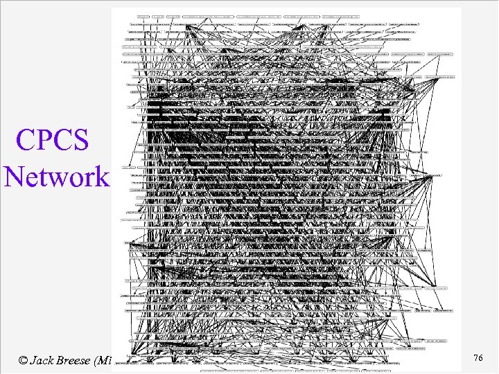
CPCS Network © Jack Breese (Microsoft) & Daphne Koller (Stanford) 76
Course Contents Concepts in Probability n Bayesian Networks n Inference » Decision making n Learning networks from data n Reasoning over time n Applications n © Jack Breese (Microsoft) & Daphne Koller (Stanford) 77
Decision making Decisions, Preferences, and Utility functions n Influence diagrams n Value of information n © Jack Breese (Microsoft) & Daphne Koller (Stanford) 78
Decision making Decision - an irrevocable allocation of domain resources n Decision should be made so as to maximize expected utility. n View decision making in terms of n u Beliefs/Uncertainties u Alternatives/Decisions u Objectives/Utilities © Jack Breese (Microsoft) & Daphne Koller (Stanford) 79
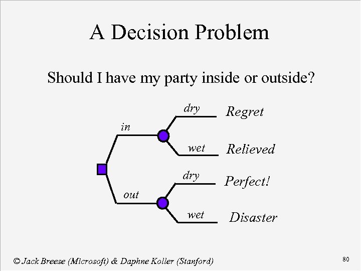
A Decision Problem Should I have my party inside or outside? dry Regret in wet dry out wet © Jack Breese (Microsoft) & Daphne Koller (Stanford) Relieved Perfect! Disaster 80
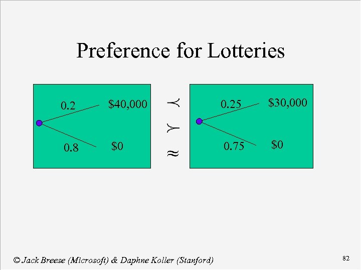
Preference for Lotteries 0. 2 $40, 000 0. 25 $30, 000 0. 8 $0 0. 75 $0 © Jack Breese (Microsoft) & Daphne Koller (Stanford) 82
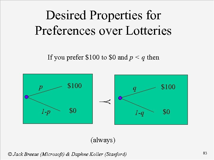
Desired Properties for Preferences over Lotteries If you prefer $100 to $0 and p < q then p $100 q $100 1 -p $0 1 -q $0 (always) © Jack Breese (Microsoft) & Daphne Koller (Stanford) 83
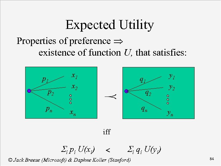
Expected Utility Properties of preference existence of function U, that satisfies: p 1 p 2 pn x 1 q 1 x 2 qn xn y 1 y 2 yn iff Si pi U(xi) Si qi U(yi) © Jack Breese (Microsoft) & Daphne Koller (Stanford) 84
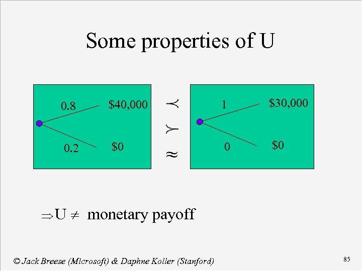
Some properties of U 0. 8 $40, 000 1 $30, 000 0. 2 $0 0 $0 U monetary payoff © Jack Breese (Microsoft) & Daphne Koller (Stanford) 85
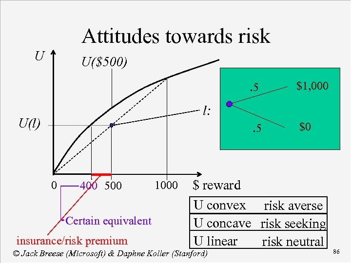
Attitudes towards risk U U($500). 5 $1, 000 . 5 $0 l: U(l) 0 400 500 Certain equivalent insurance/risk premium 1000 $ reward U convex risk averse U concave risk seeking U linear risk neutral © Jack Breese (Microsoft) & Daphne Koller (Stanford) 86
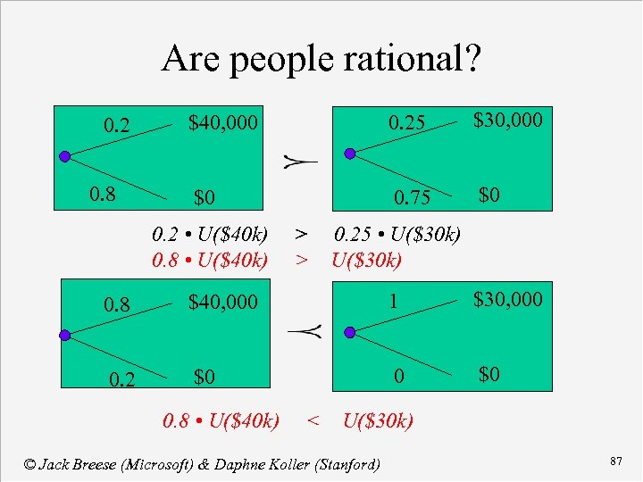
Are people rational? 0. 2 0. 8 $40, 000 0. 25 $30, 000 $0 0. 75 $0 0. 2 • U($40 k) 0. 8 • U($40 k) > 0. 25 • U($30 k) > U($30 k) 0. 8 $40, 000 1 $30, 000 0. 2 $0 0. 8 • U($40 k) < U($30 k) © Jack Breese (Microsoft) & Daphne Koller (Stanford) 87
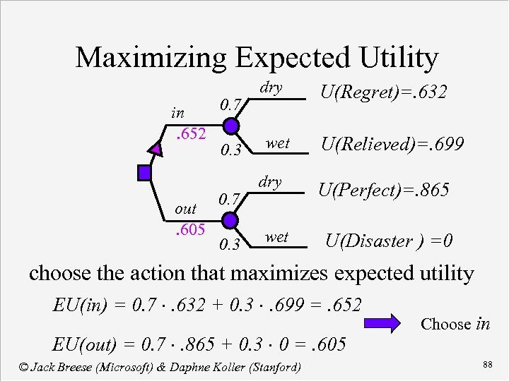
Maximizing Expected Utility 0. 7 in. 652 0. 3 out. 605 0. 7 0. 3 dry wet U(Regret)=. 632 U(Relieved)=. 699 U(Perfect)=. 865 U(Disaster ) =0 choose the action that maximizes expected utility EU(in) = 0. 7 ×. 632 + 0. 3 ×. 699 =. 652 EU(out) = 0. 7 ×. 865 + 0. 3 × 0 =. 605 © Jack Breese (Microsoft) & Daphne Koller (Stanford) Choose in 88
Multi-attribute utilities (or: Money isn’t everything) n Many aspects of an outcome combine to determine our preferences. u vacation planning: cost, flying time, beach quality, food quality, … u medical decision making: risk of death (micromort), quality of life (QALY), cost of treatment, … n For rational decision making, must combine all relevant factors into single utility function. © Jack Breese (Microsoft) & Daphne Koller (Stanford) 89
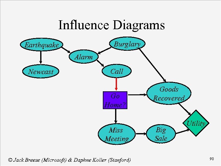
Influence Diagrams Burglary Earthquake Alarm Newcast Call Go Home? Miss Meeting © Jack Breese (Microsoft) & Daphne Koller (Stanford) Goods Recovered Big Sale Utility 90
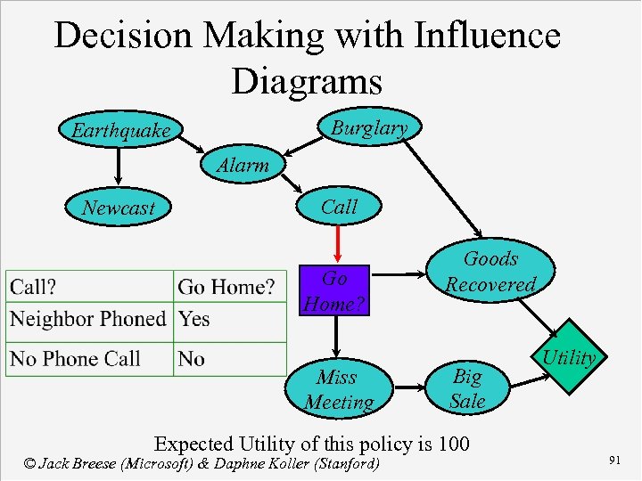
Decision Making with Influence Diagrams Burglary Earthquake Alarm Newcast Call Go Home? Miss Meeting Goods Recovered Big Sale Expected Utility of this policy is 100 © Jack Breese (Microsoft) & Daphne Koller (Stanford) Utility 91
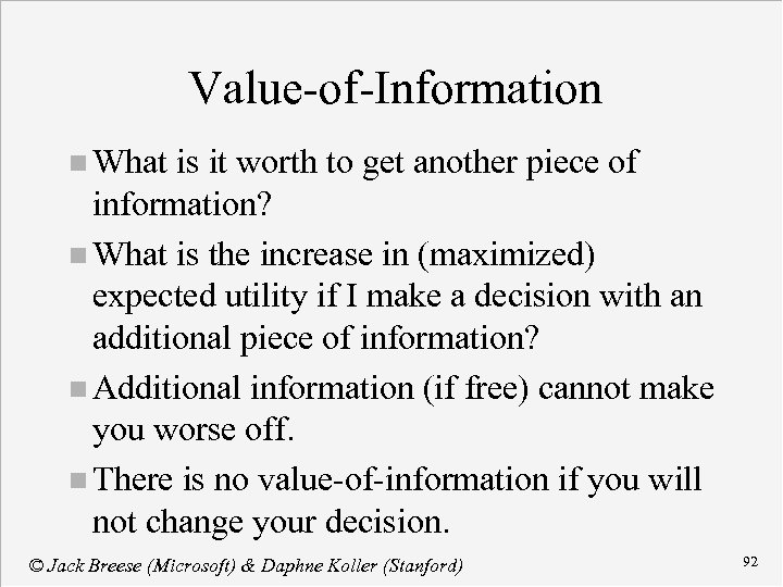
Value-of-Information n What is it worth to get another piece of information? n What is the increase in (maximized) expected utility if I make a decision with an additional piece of information? n Additional information (if free) cannot make you worse off. n There is no value-of-information if you will not change your decision. © Jack Breese (Microsoft) & Daphne Koller (Stanford) 92
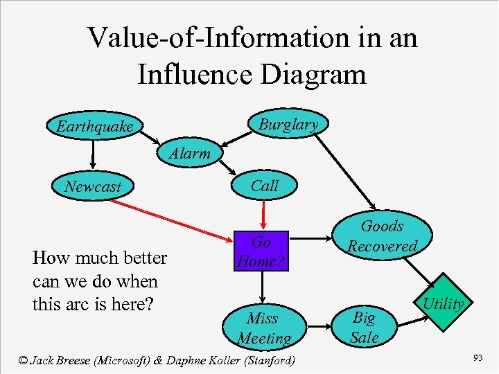
Value-of-Information in an Influence Diagram Burglary Earthquake Alarm Newcast How much better can we do when this arc is here? Call Go Home? Miss Meeting © Jack Breese (Microsoft) & Daphne Koller (Stanford) Goods Recovered Big Sale Utility 93
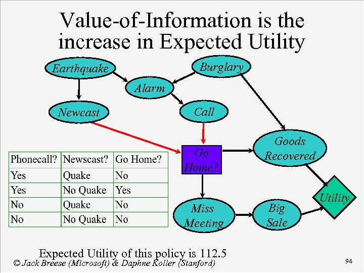
Value-of-Information is the increase in Expected Utility Burglary Earthquake Alarm Newcast Call Go Home? Miss Meeting Expected Utility of this policy is 112. 5 © Jack Breese (Microsoft) & Daphne Koller (Stanford) Goods Recovered Big Sale Utility 94
Course Contents Concepts in Probability n Bayesian Networks n Inference n Decision making » Learning networks from data n Reasoning over time n Applications n © Jack Breese (Microsoft) & Daphne Koller (Stanford) 95
Learning networks from data The learning task n Parameter learning n u Fully observable u Partially observable Structure learning n Hidden variables n © Jack Breese (Microsoft) & Daphne Koller (Stanford) 96
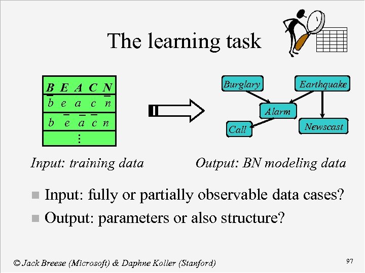
The learning task Burglary B E A C N b e a c n Alarm b e a c n Call . . . Input: training data Earthquake Newscast Output: BN modeling data Input: fully or partially observable data cases? n Output: parameters or also structure? n © Jack Breese (Microsoft) & Daphne Koller (Stanford) 97
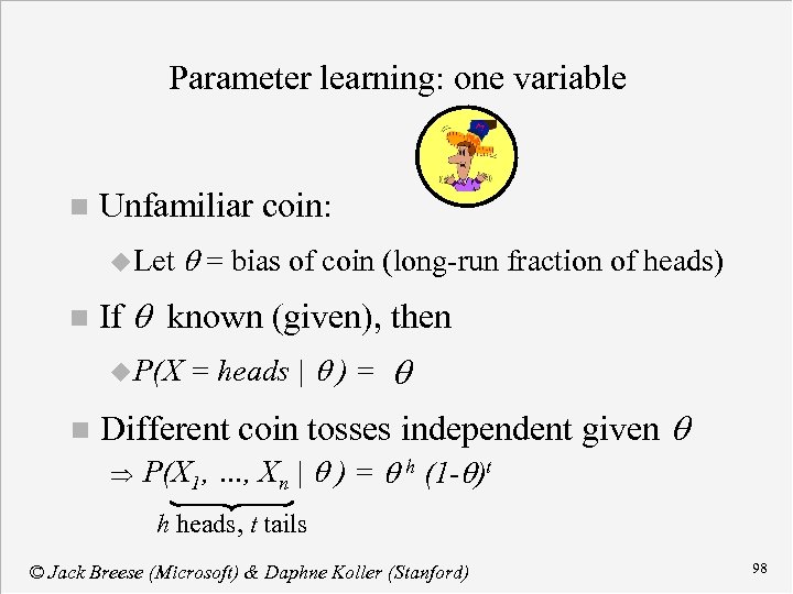
Parameter learning: one variable n Unfamiliar coin: u Let n If q known (given), then u P(X n q = bias of coin (long-run fraction of heads) = heads | q ) = q Different coin tosses independent given q P(X 1, …, Xn | q ) = q h (1 -q)t h heads, t tails © Jack Breese (Microsoft) & Daphne Koller (Stanford) 98
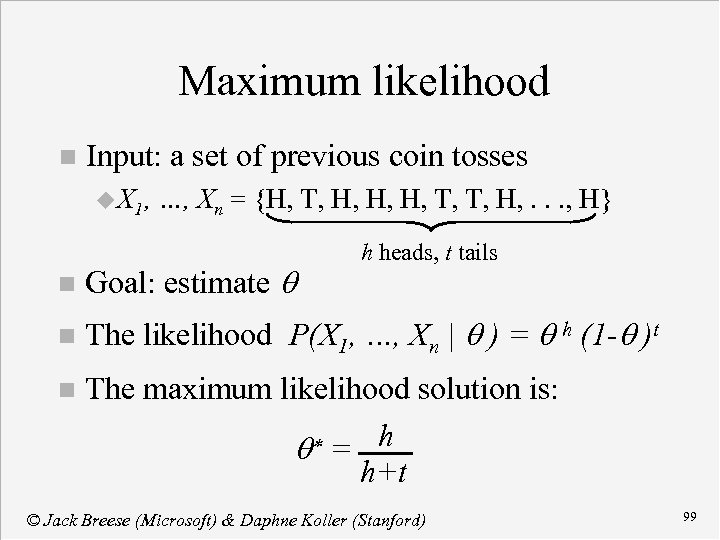
Maximum likelihood n Input: a set of previous coin tosses u X 1, …, Xn = {H, T, H, H, H, T, T, H, . . . , H} h heads, t tails n Goal: estimate q n The likelihood P(X 1, …, Xn | q ) = q h (1 -q )t n The maximum likelihood solution is: q* = h h+t © Jack Breese (Microsoft) & Daphne Koller (Stanford) 99
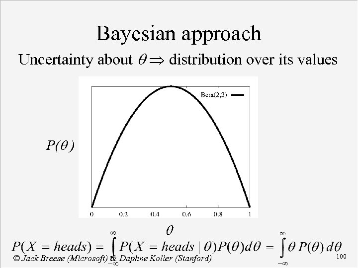
Bayesian approach Uncertainty about q distribution over its values P(q ) q © Jack Breese (Microsoft) & Daphne Koller (Stanford) 100
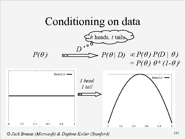
Conditioning on data h heads, t tails P(q ) D P(q | D) P(q ) P(D | q ) = P(q ) q h (1 -q )t 1 head 1 tail © Jack Breese (Microsoft) & Daphne Koller (Stanford) 101
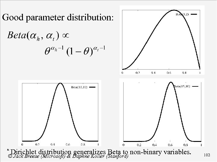
Good parameter distribution: * Dirichlet distribution generalizes Beta to non-binary variables. © Jack Breese (Microsoft) & Daphne Koller (Stanford) 102
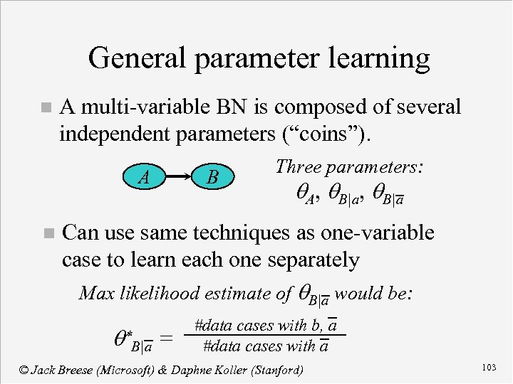
General parameter learning n A multi-variable BN is composed of several independent parameters (“coins”). A n B Three parameters: q. A, q. B|a Can use same techniques as one-variable case to learn each one separately Max likelihood estimate of q. B|a would be: q* B|a = #data cases with b, a #data cases with a © Jack Breese (Microsoft) & Daphne Koller (Stanford) 103
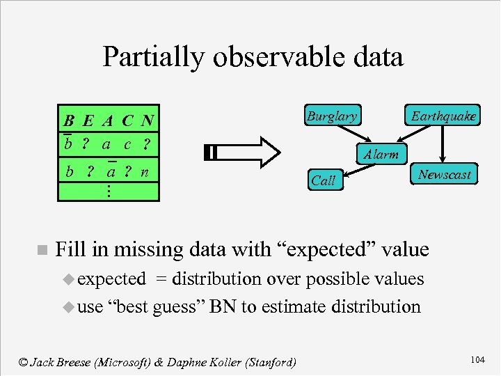
Partially observable data B E A C N b ? a c ? b ? a ? n . . . n Burglary Earthquake Alarm Call Newscast Fill in missing data with “expected” value u expected = distribution over possible values u use “best guess” BN to estimate distribution © Jack Breese (Microsoft) & Daphne Koller (Stanford) 104
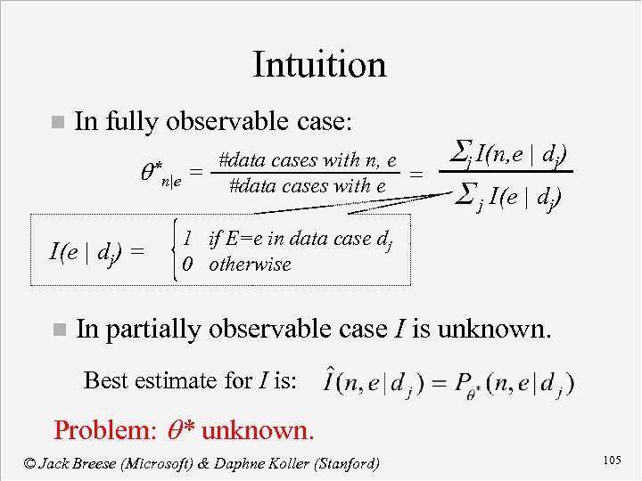
Intuition n In fully observable case: #data cases with n, e n|e = #data cases with e = q* I(e | dj) = n Sj I(n, e | dj) S j I(e | dj) 1 if E=e in data case dj 0 otherwise In partially observable case I is unknown. Best estimate for I is: Problem: q* unknown. © Jack Breese (Microsoft) & Daphne Koller (Stanford) 105
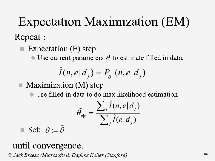
Expectation Maximization (EM) Repeat : n Expectation (E) step u Use n Maximization (M) step u Use n current parameters q to estimate filled in data to do max likelihood estimation Set: until convergence. © Jack Breese (Microsoft) & Daphne Koller (Stanford) 106
Structure learning Goal: find “good” BN structure (relative to data) Solution: do heuristic search over space of network structures. © Jack Breese (Microsoft) & Daphne Koller (Stanford) 107
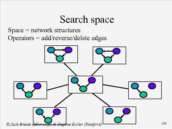
Search space Space = network structures Operators = add/reverse/delete edges © Jack Breese (Microsoft) & Daphne Koller (Stanford) 108
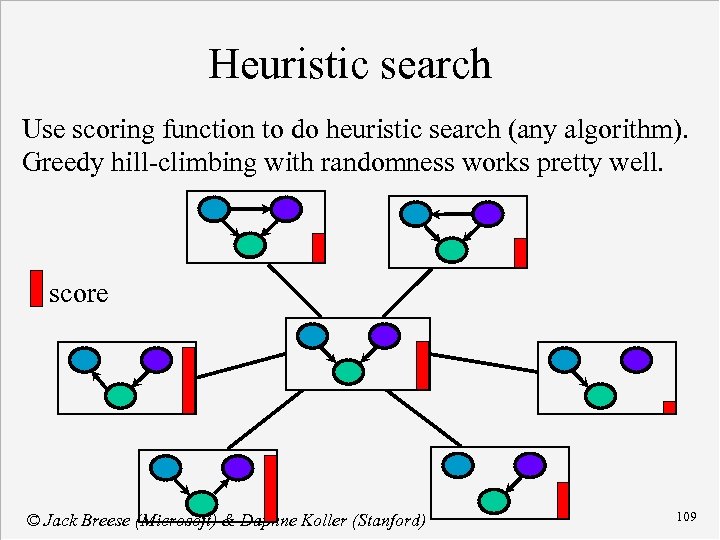
Heuristic search Use scoring function to do heuristic search (any algorithm). Greedy hill-climbing with randomness works pretty well. score © Jack Breese (Microsoft) & Daphne Koller (Stanford) 109
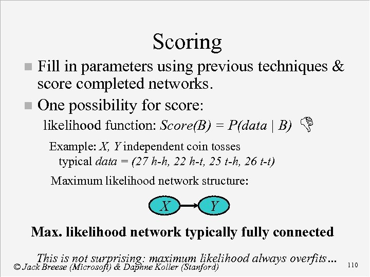
Scoring Fill in parameters using previous techniques & score completed networks. n One possibility for score: n likelihood function: Score(B) = P(data | B) D Example: X, Y independent coin tosses typical data = (27 h-h, 22 h-t, 25 t-h, 26 t-t) Maximum likelihood network structure: X Y Max. likelihood network typically fully connected This is not surprising: maximum likelihood always overfits… © Jack Breese (Microsoft) & Daphne Koller (Stanford) 110
Better scoring functions n MDL formulation: balance fit to data and model complexity (# of parameters) Score(B) = P(data | B) - model complexity n Full Bayesian formulation u prior on network structures & parameters u more parameters higher dimensional space u get balance effect as a byproduct* * with Dirichlet parameter prior, MDL is an approximation to full Bayesian score. © Jack Breese (Microsoft) & Daphne Koller (Stanford) 111
Hidden variables n There may be interesting variables that we never get to observe: u topic of a document in information retrieval; u user’s current task in online help system. n Our learning algorithm should u hypothesize the existence of such variables; u learn an appropriate state space for them. © Jack Breese (Microsoft) & Daphne Koller (Stanford) 112
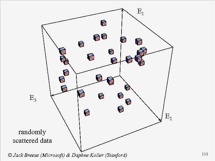
E 1 E 3 E 2 randomly scattered data © Jack Breese (Microsoft) & Daphne Koller (Stanford) 113
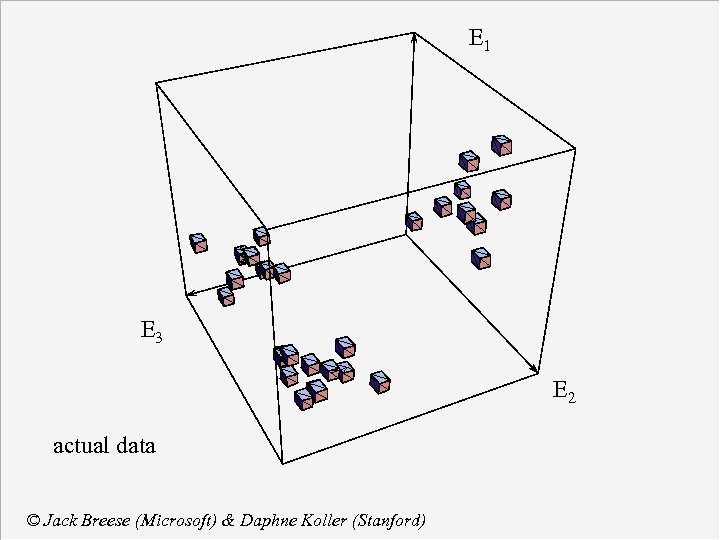
E 1 E 3 E 2 actual data © Jack Breese (Microsoft) & Daphne Koller (Stanford)
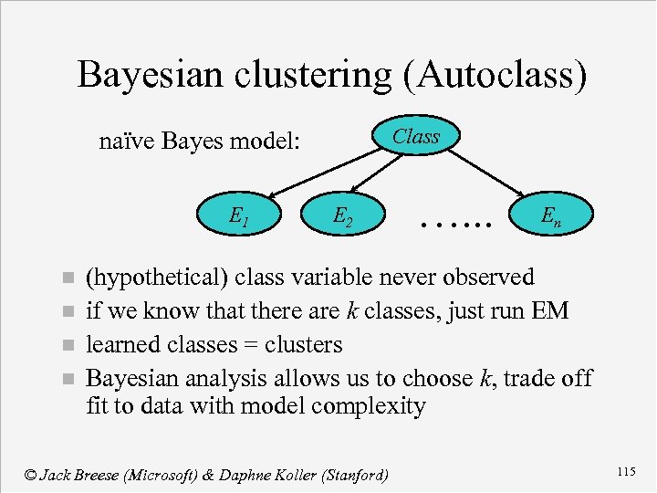
Bayesian clustering (Autoclass) Class naïve Bayes model: E 1 n n E 2 …. . . En (hypothetical) class variable never observed if we know that there are k classes, just run EM learned classes = clusters Bayesian analysis allows us to choose k, trade off fit to data with model complexity © Jack Breese (Microsoft) & Daphne Koller (Stanford) 115
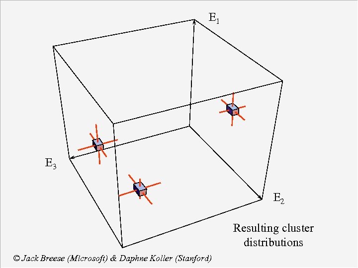
E 1 E 3 E 2 Resulting cluster distributions © Jack Breese (Microsoft) & Daphne Koller (Stanford)
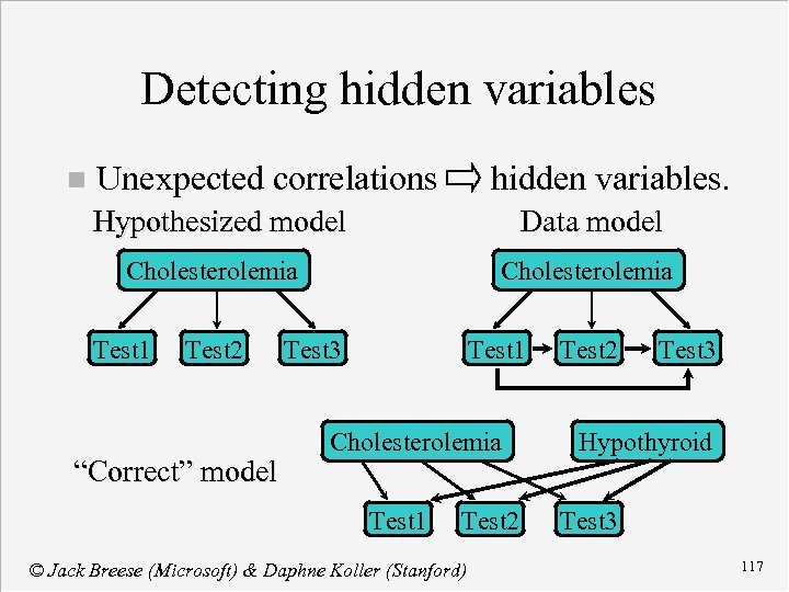
Detecting hidden variables n Unexpected correlations hidden variables. Hypothesized model Data model Cholesterolemia Test 1 Test 2 “Correct” model Cholesterolemia Test 3 Test 1 Cholesterolemia Test 1 Test 2 © Jack Breese (Microsoft) & Daphne Koller (Stanford) Test 2 Test 3 Hypothyroid Test 3 117
Course Contents Concepts in Probability n Bayesian Networks n Inference n Decision making n Learning networks from data » Reasoning over time n Applications n © Jack Breese (Microsoft) & Daphne Koller (Stanford) 118
Reasoning over time Dynamic Bayesian networks n Hidden Markov models n Decision-theoretic planning n u Markov decision problems u Structured representation of actions u The qualification problem & the frame problem u Causality (and the frame problem revisited) © Jack Breese (Microsoft) & Daphne Koller (Stanford) 119
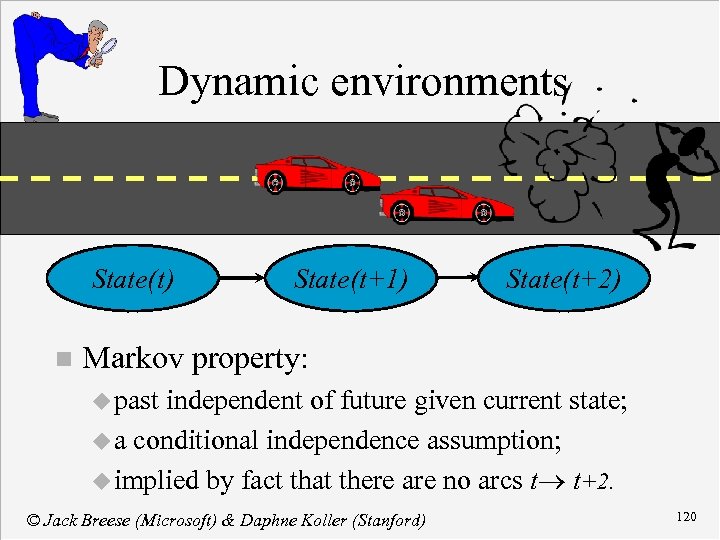
Dynamic environments State(t) n State(t+1) State(t+2) Markov property: u past independent of future given current state; u a conditional independence assumption; u implied by fact that there are no arcs t t+2. © Jack Breese (Microsoft) & Daphne Koller (Stanford) 120
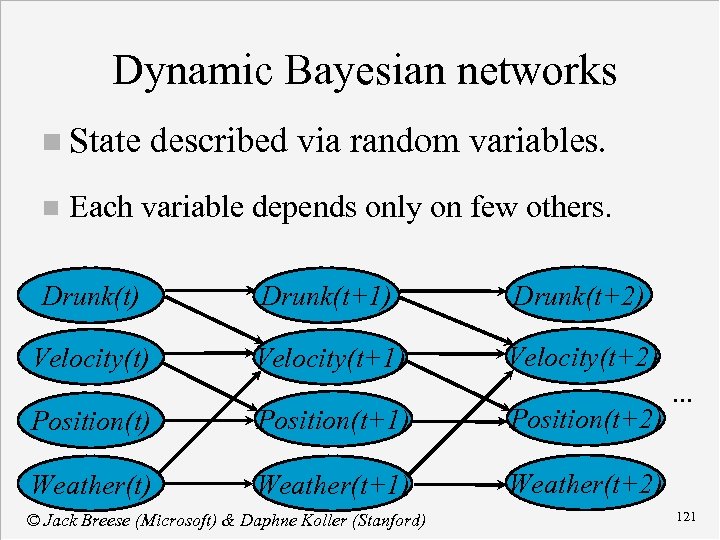
Dynamic Bayesian networks n State n described via random variables. Each variable depends only on few others. Drunk(t) Drunk(t+1) Drunk(t+2) Velocity(t+1) Velocity(t+2) Position(t+1) Position(t+2) Weather(t+1) . . . Weather(t+2) © Jack Breese (Microsoft) & Daphne Koller (Stanford) 121
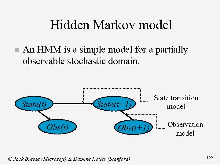
Hidden Markov model n An HMM is a simple model for a partially observable stochastic domain. State(t) Obs(t) State(t+1) Obs(t+1) © Jack Breese (Microsoft) & Daphne Koller (Stanford) State transition model Observation model 122
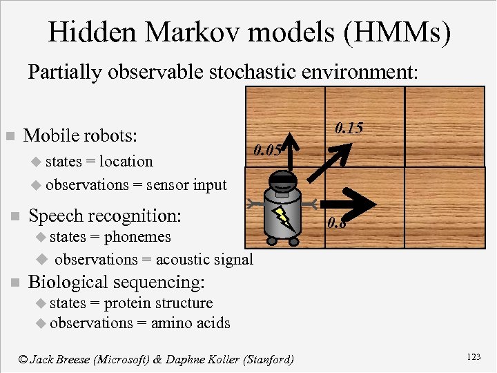
Hidden Markov models (HMMs) Partially observable stochastic environment: Mobile robots: n u states = location u observations = sensor input n 0. 15 0. 05 Speech recognition: u states = phonemes u observations = acoustic signal n 0. 8 Biological sequencing: u states = protein structure u observations = amino acids © Jack Breese (Microsoft) & Daphne Koller (Stanford) 123
HMMs and DBNs HMMs are just very simple DBNs. n Standard inference & learning algorithms for HMMs are instances of DBN algorithms n u Forward-backward = polytree u Baum-Welch = EM u Viterbi = most probable explanation. © Jack Breese (Microsoft) & Daphne Koller (Stanford) 124
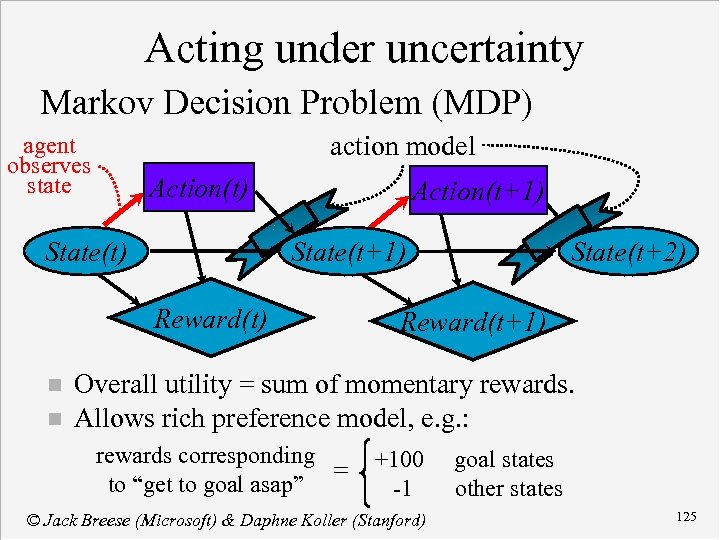
Acting under uncertainty Markov Decision Problem (MDP) action model agent observes state Action(t) State(t) Action(t+1) State(t+1) Reward(t) n n State(t+2) Reward(t+1) Overall utility = sum of momentary rewards. Allows rich preference model, e. g. : rewards corresponding = to “get to goal asap” +100 -1 © Jack Breese (Microsoft) & Daphne Koller (Stanford) goal states other states 125
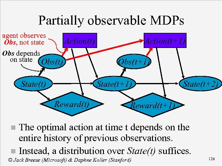
Partially observable MDPs agent observes Action(t) Obs, not state Obs depends on state Obs(t) State(t) Action(t+1) Obs(t+1) State(t+1) Reward(t) State(t+2) Reward(t+1) The optimal action at time t depends on the entire history of previous observations. n Instead, a distribution over State(t) suffices. n © Jack Breese (Microsoft) & Daphne Koller (Stanford) 126
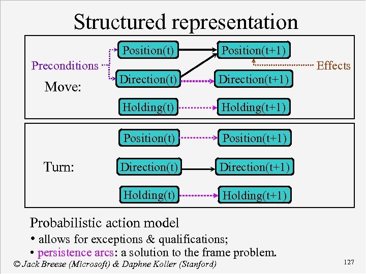
Structured representation Position(t) Position(t+1) Preconditions Effects Holding(t+1) Position(t+1) Direction(t+1) Holding(t) Turn: Direction(t+1) Holding(t) Move: Direction(t) Holding(t+1) Probabilistic action model • allows for exceptions & qualifications; • persistence arcs: a solution to the frame problem. © Jack Breese (Microsoft) & Daphne Koller (Stanford) 127
Causality Modeling the effects of interventions n Observing vs. “setting” a variable n A form of persistence modeling n © Jack Breese (Microsoft) & Daphne Koller (Stanford) 128
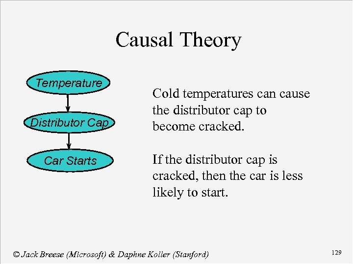
Causal Theory Temperature Distributor Cap Car Starts Cold temperatures can cause the distributor cap to become cracked. If the distributor cap is cracked, then the car is less likely to start. © Jack Breese (Microsoft) & Daphne Koller (Stanford) 129
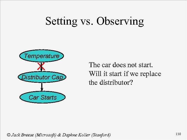
Setting vs. Observing Temperature Distributor Cap The car does not start. Will it start if we replace the distributor? Car Starts © Jack Breese (Microsoft) & Daphne Koller (Stanford) 130
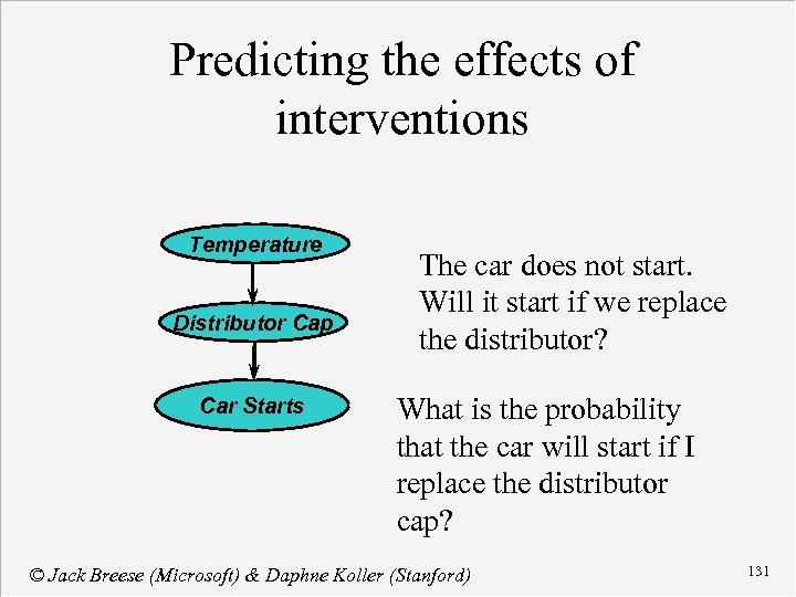
Predicting the effects of interventions Temperature Distributor Cap Car Starts The car does not start. Will it start if we replace the distributor? What is the probability that the car will start if I replace the distributor cap? © Jack Breese (Microsoft) & Daphne Koller (Stanford) 131
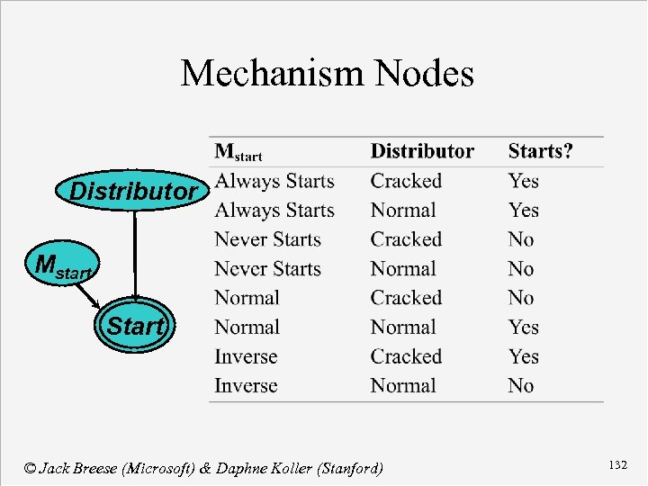
Mechanism Nodes Distributor Mstart Start © Jack Breese (Microsoft) & Daphne Koller (Stanford) 132
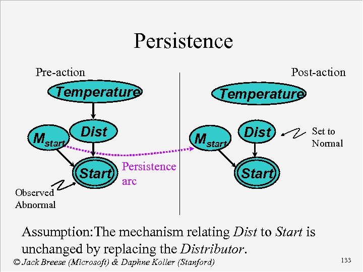
Persistence Pre-action Post-action Temperature Dist Mstart Observed Abnormal Mstart Persistence Start arc Set to Normal Start Assumption: The mechanism relating Dist to Start is unchanged by replacing the Distributor. © Jack Breese (Microsoft) & Daphne Koller (Stanford) 133
Course Contents Concepts in Probability n Bayesian Networks n Inference n Decision making n Learning networks from data n Reasoning over time » Applications n © Jack Breese (Microsoft) & Daphne Koller (Stanford) 134
Applications n Medical expert systems u Pathfinder u Parenting n MSN Fault diagnosis u Ricoh FIXIT u Decision-theoretic troubleshooting Vista n Collaborative filtering n © Jack Breese (Microsoft) & Daphne Koller (Stanford) 135
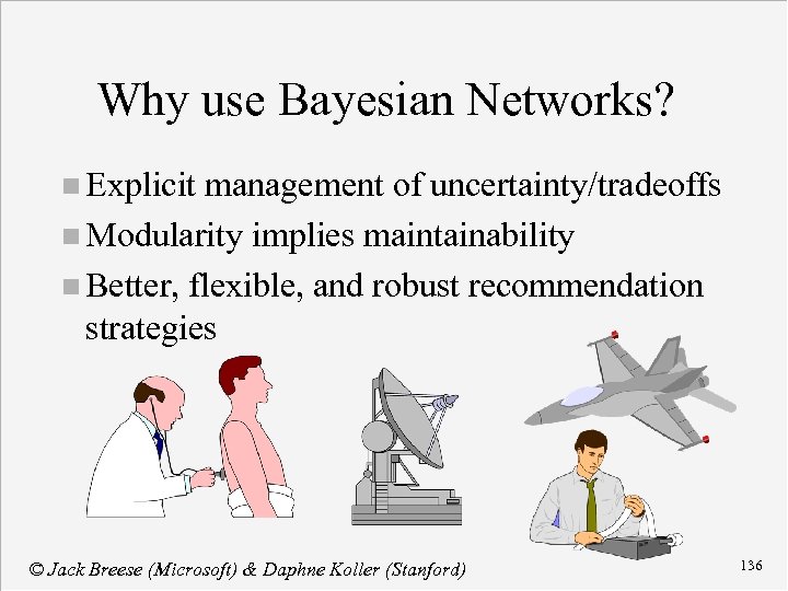
Why use Bayesian Networks? n Explicit management of uncertainty/tradeoffs n Modularity implies maintainability n Better, flexible, and robust recommendation strategies © Jack Breese (Microsoft) & Daphne Koller (Stanford) 136
Pathfinder is one of the first BN systems. n It performs diagnosis of lymph-node diseases. n It deals with over 60 diseases and 100 findings. n Commercialized by Intellipath and Chapman Hall publishing and applied to about 20 tissue types. n © Jack Breese (Microsoft) & Daphne Koller (Stanford) 137
Studies of Pathfinder Diagnostic Performance Naïve Bayes performed considerably better than certainty factors and Dempster-Shafer Belief Functions. n Incorrect zero probabilities caused 10% of cases to be misdiagnosed. n Full Bayesian network model with feature dependencies did best. n © Jack Breese (Microsoft) & Daphne Koller (Stanford) 138
On Parenting: Selecting problem n n n Diagnostic indexing for Home Health site on Microsoft Network Enter symptoms for pediatric complaints Recommends multimedia content © Jack Breese (Microsoft) & Daphne Koller (Stanford) 140
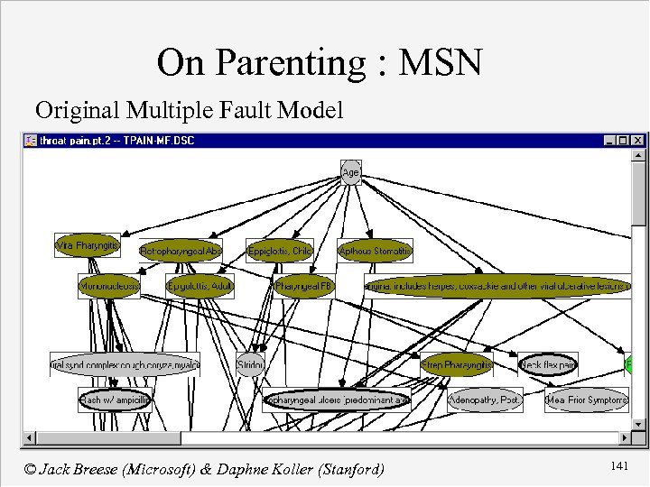
On Parenting : MSN Original Multiple Fault Model © Jack Breese (Microsoft) & Daphne Koller (Stanford) 141
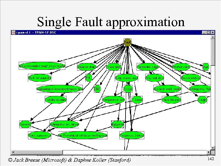
Single Fault approximation © Jack Breese (Microsoft) & Daphne Koller (Stanford) 142
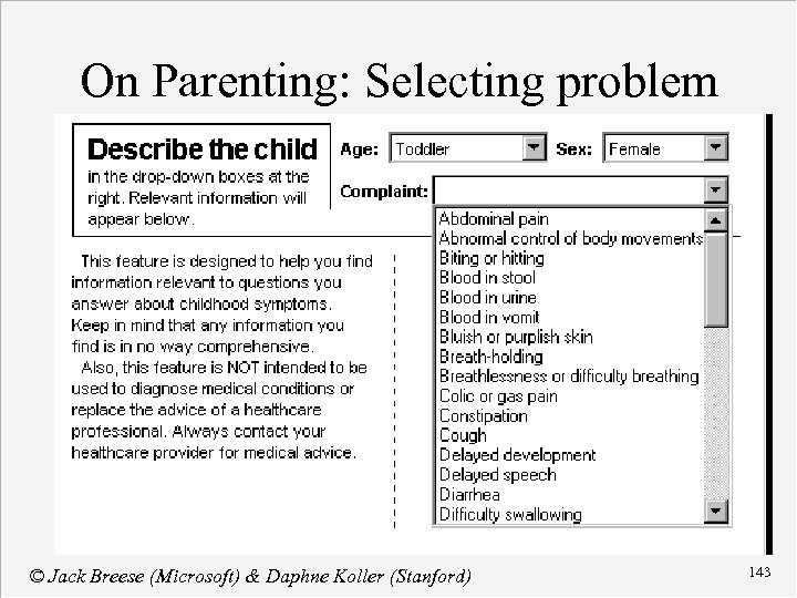
On Parenting: Selecting problem © Jack Breese (Microsoft) & Daphne Koller (Stanford) 143
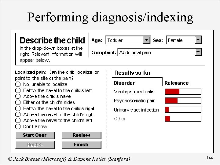
Performing diagnosis/indexing © Jack Breese (Microsoft) & Daphne Koller (Stanford) 144
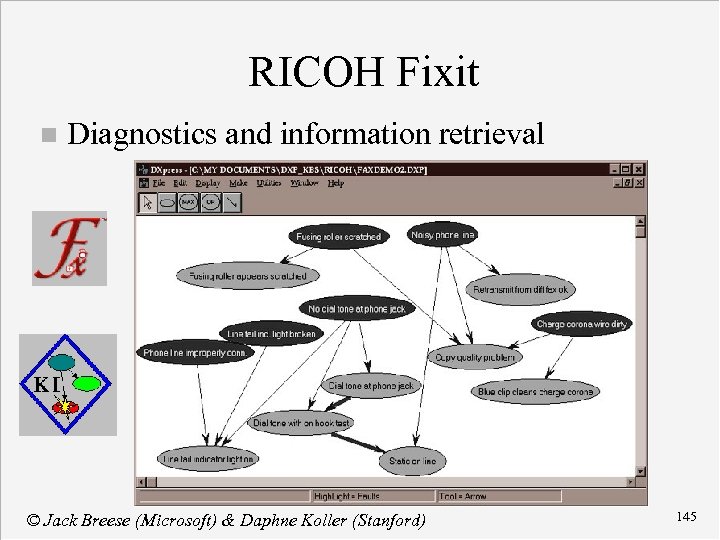
RICOH Fixit n Diagnostics and information retrieval © Jack Breese (Microsoft) & Daphne Koller (Stanford) 145
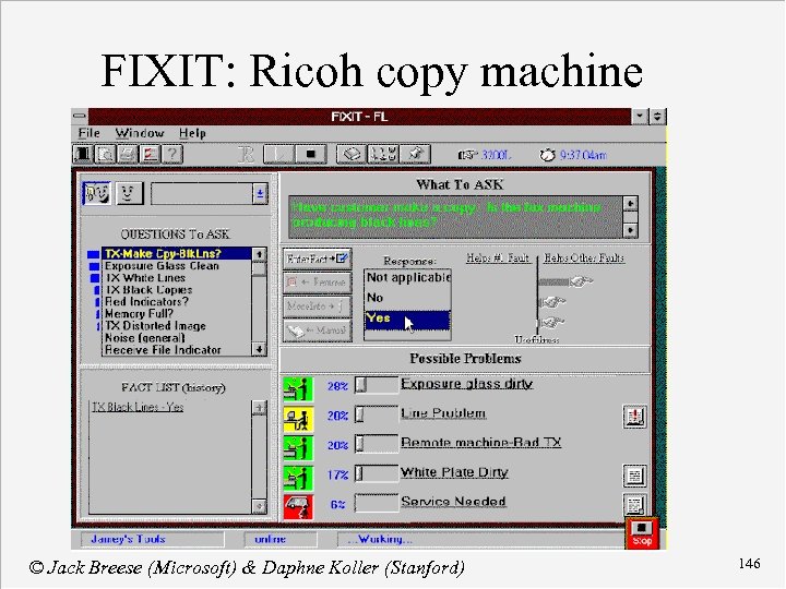
FIXIT: Ricoh copy machine © Jack Breese (Microsoft) & Daphne Koller (Stanford) 146
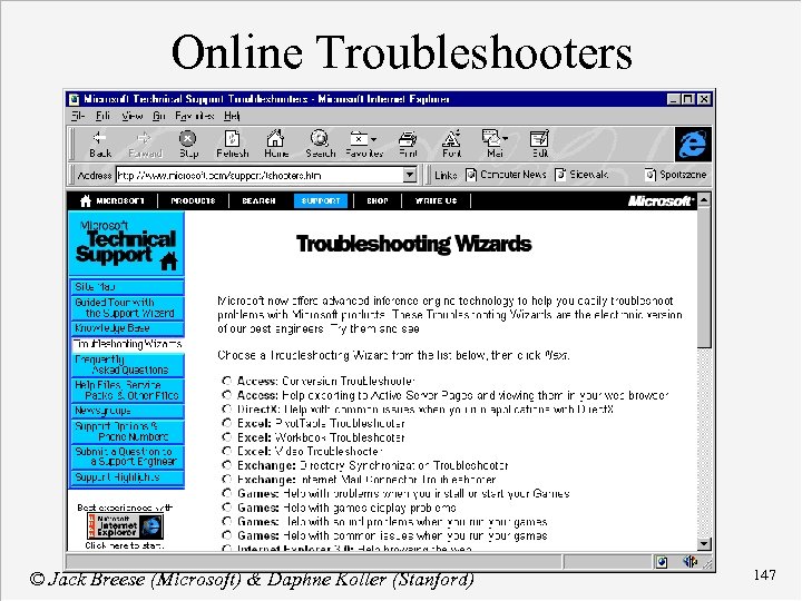
Online Troubleshooters © Jack Breese (Microsoft) & Daphne Koller (Stanford) 147
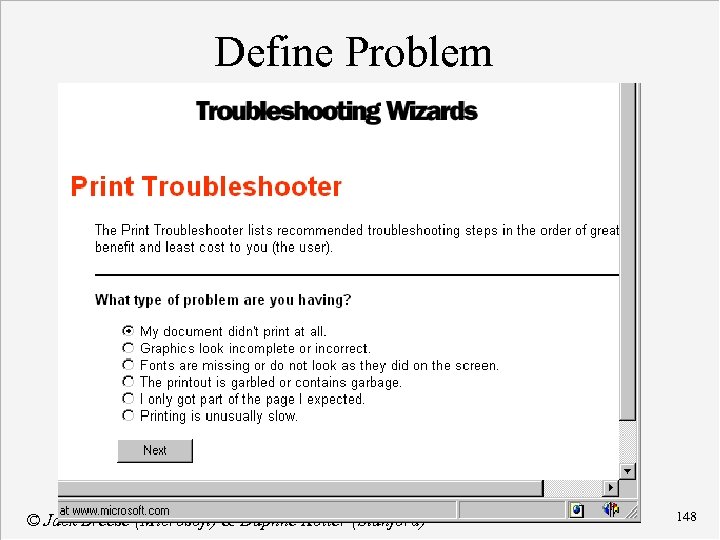
Define Problem © Jack Breese (Microsoft) & Daphne Koller (Stanford) 148
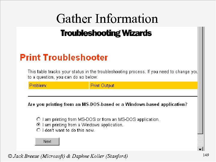
Gather Information © Jack Breese (Microsoft) & Daphne Koller (Stanford) 149
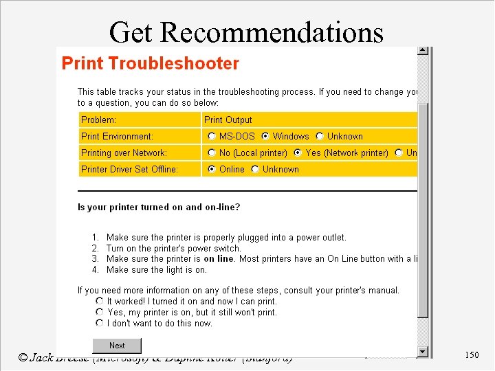
Get Recommendations © Jack Breese (Microsoft) & Daphne Koller (Stanford) 150
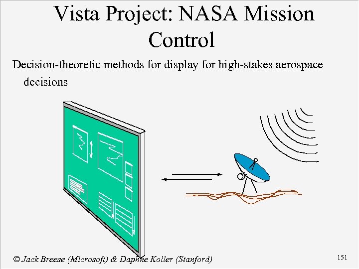
Vista Project: NASA Mission Control Decision-theoretic methods for display for high-stakes aerospace decisions © Jack Breese (Microsoft) & Daphne Koller (Stanford) 151
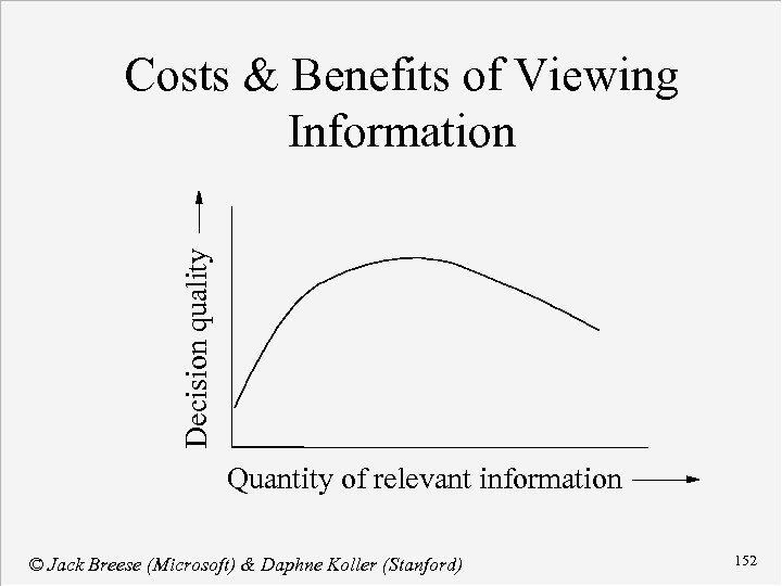
Decision quality Costs & Benefits of Viewing Information Quantity of relevant information © Jack Breese (Microsoft) & Daphne Koller (Stanford) 152
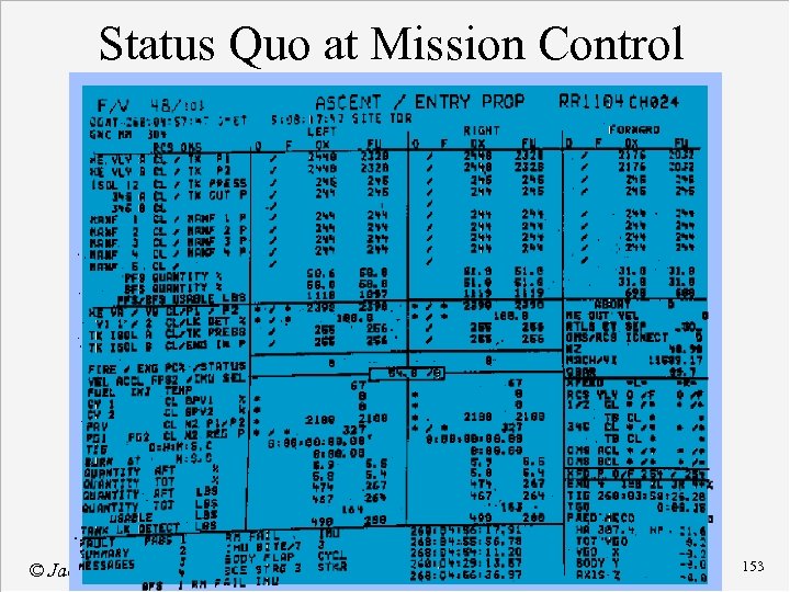
Status Quo at Mission Control © Jack Breese (Microsoft) & Daphne Koller (Stanford) 153
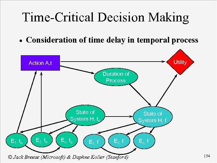
Time-Critical Decision Making · Consideration of time delay in temporal process Utility Action A, t Duration of Process State of System H, to E 1, to E 2, to En, to E 1, t’ State of System H, t’ E 2, t’ © Jack Breese (Microsoft) & Daphne Koller (Stanford) En, t’ 154
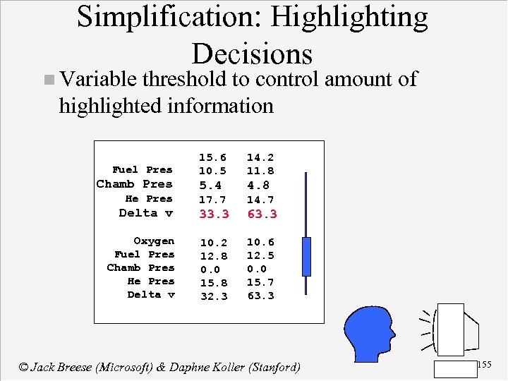
Simplification: Highlighting Decisions n Variable threshold to control amount of highlighted information Oxygen Fuel Pres Chamb Pres He Pres Delta v 15. 6 10. 5 14. 2 11. 8 5. 4 4. 8 17. 7 14. 7 33. 3 63. 3 10. 2 12. 8 0. 0 15. 8 32. 3 10. 6 12. 5 0. 0 15. 7 63. 3 © Jack Breese (Microsoft) & Daphne Koller (Stanford) 155
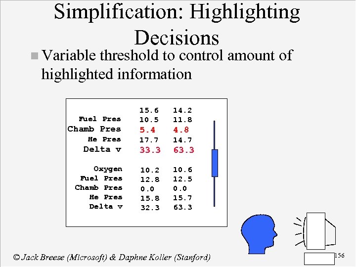
Simplification: Highlighting Decisions n Variable threshold to control amount of highlighted information Oxygen Fuel Pres Chamb Pres He Pres Delta v 15. 6 10. 5 14. 2 11. 8 5. 4 4. 8 17. 7 14. 7 33. 3 63. 3 10. 2 12. 8 0. 0 15. 8 32. 3 10. 6 12. 5 0. 0 15. 7 63. 3 © Jack Breese (Microsoft) & Daphne Koller (Stanford) 156
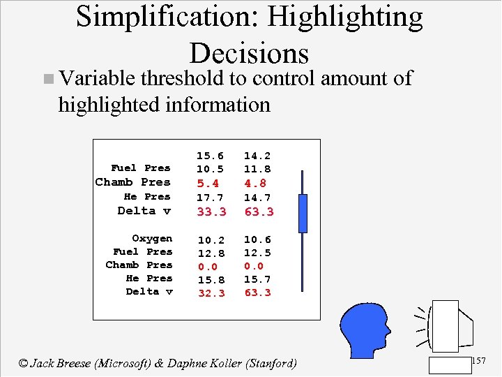
Simplification: Highlighting Decisions n Variable threshold to control amount of highlighted information Oxygen Fuel Pres Chamb Pres He Pres Delta v 15. 6 10. 5 14. 2 11. 8 5. 4 4. 8 17. 7 14. 7 33. 3 63. 3 10. 2 12. 8 0. 0 15. 8 32. 3 10. 6 12. 5 0. 0 15. 7 63. 3 © Jack Breese (Microsoft) & Daphne Koller (Stanford) 157
What is Collaborative Filtering? A way to find cool websites, news stories, music artists etc n Uses data on the preferences of many users, not descriptions of the content. n Firefly, Net Perceptions (Group. Lens), and others offer this technology. n © Jack Breese (Microsoft) & Daphne Koller (Stanford) 158
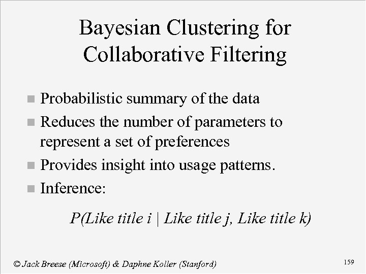
Bayesian Clustering for Collaborative Filtering Probabilistic summary of the data n Reduces the number of parameters to represent a set of preferences n Provides insight into usage patterns. n Inference: n P(Like title i | Like title j, Like title k) © Jack Breese (Microsoft) & Daphne Koller (Stanford) 159
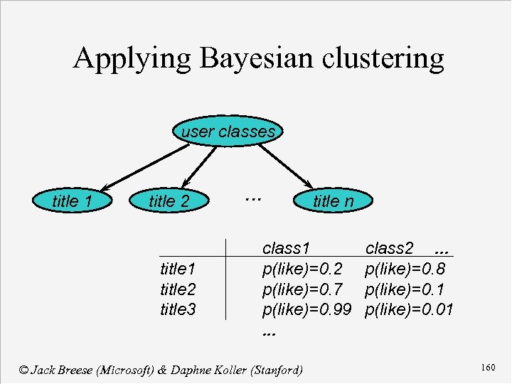
Applying Bayesian clustering user classes title 1 title 2 title 3 . . . title n class 1 p(like)=0. 2 p(like)=0. 7 p(like)=0. 99. . . © Jack Breese (Microsoft) & Daphne Koller (Stanford) class 2. . . p(like)=0. 8 p(like)=0. 1 p(like)=0. 01 160
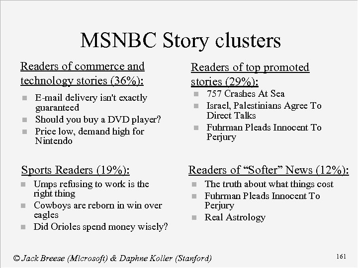
MSNBC Story clusters Readers of commerce and technology stories (36%): n n n E-mail delivery isn't exactly guaranteed Should you buy a DVD player? Price low, demand high for Nintendo Sports Readers (19%): n n n Umps refusing to work is the right thing Cowboys are reborn in win over eagles Did Orioles spend money wisely? Readers of top promoted stories (29%): n n n 757 Crashes At Sea Israel, Palestinians Agree To Direct Talks Fuhrman Pleads Innocent To Perjury Readers of “Softer” News (12%): n n n The truth about what things cost Fuhrman Pleads Innocent To Perjury Real Astrology © Jack Breese (Microsoft) & Daphne Koller (Stanford) 161
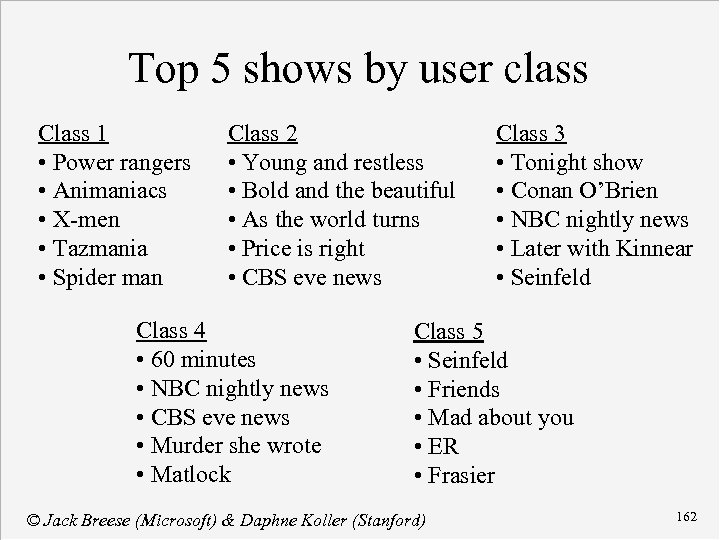
Top 5 shows by user class Class 1 • Power rangers • Animaniacs • X-men • Tazmania • Spider man Class 2 • Young and restless • Bold and the beautiful • As the world turns • Price is right • CBS eve news Class 4 • 60 minutes • NBC nightly news • CBS eve news • Murder she wrote • Matlock Class 3 • Tonight show • Conan O’Brien • NBC nightly news • Later with Kinnear • Seinfeld Class 5 • Seinfeld • Friends • Mad about you • ER • Frasier © Jack Breese (Microsoft) & Daphne Koller (Stanford) 162
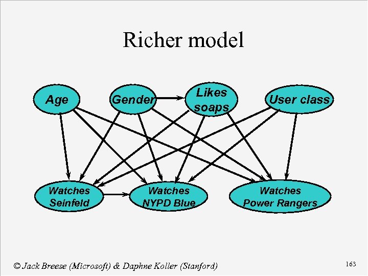
Richer model Age Watches Seinfeld Gender Likes soaps Watches NYPD Blue © Jack Breese (Microsoft) & Daphne Koller (Stanford) User class Watches Power Rangers 163
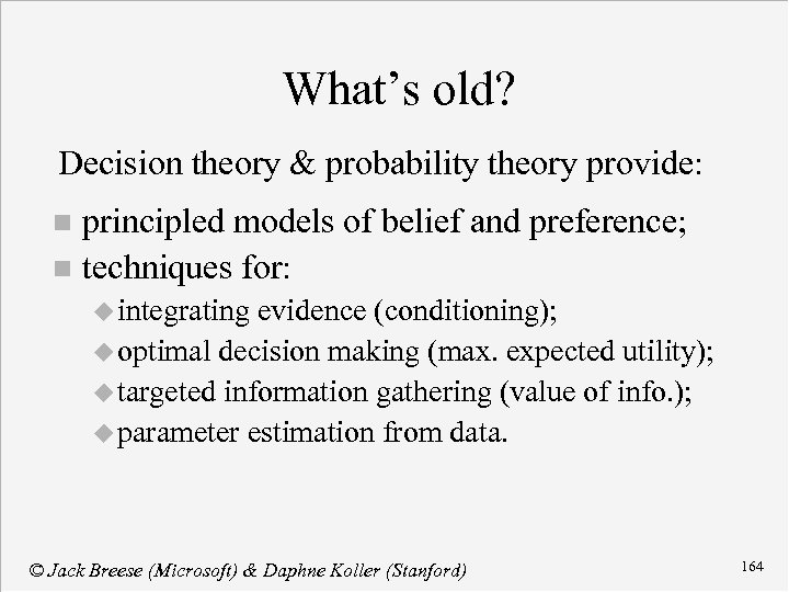
What’s old? Decision theory & probability theory provide: principled models of belief and preference; n techniques for: n u integrating evidence (conditioning); u optimal decision making (max. expected utility); u targeted information gathering (value of info. ); u parameter estimation from data. © Jack Breese (Microsoft) & Daphne Koller (Stanford) 164
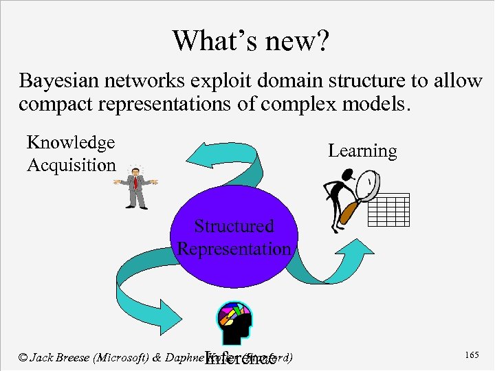
What’s new? Bayesian networks exploit domain structure to allow compact representations of complex models. Knowledge Acquisition Learning Structured Representation © Jack Breese (Microsoft) & Daphne. Inference Koller (Stanford) 165
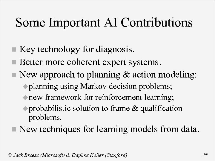
Some Important AI Contributions Key technology for diagnosis. n Better more coherent expert systems. n New approach to planning & action modeling: n u planning using Markov decision problems; u new framework for reinforcement learning; u probabilistic solution to frame & qualification problems. n New techniques for learning models from data. © Jack Breese (Microsoft) & Daphne Koller (Stanford) 166
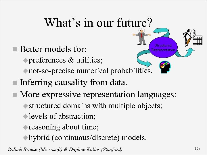
What’s in our future? n Better models for: Structured Representation u preferences & utilities; u not-so-precise numerical probabilities. Inferring causality from data. n More expressive representation languages: n u structured domains with multiple objects; u levels of abstraction; u reasoning about time; u hybrid (continuous/discrete) models. © Jack Breese (Microsoft) & Daphne Koller (Stanford) 167
db4932f388cd0b3f03dadc3c12e319f4.ppt