f2bae6bf5463b95d064019dcb97c294d.ppt
- Количество слайдов: 76


Tubas ELECTRICAL NETWORK STUDY Prepared by : Omar Abu-Omar Ahmad Nerat Sameed banifadel PRESENTATION TO: Dr. MAHER KHAMASH

Contents : • Chapter 1 : Introduction • • 1. 1 Improvement the distribution of electrical network 1. 2 Methods of improvement of distribution electrical networks • Chapter 2 : Tubas City Electricity Network • • 2. 1 Electrical Supply 2. 2 Elements Of The Network 2. 3 Electrical Consumption 2. 4 Problems in The Network • • • Chapter 3 : Load Flow Analysis Chapter 4 : Maximum Case Chapter 5 : Minimum Case Chapter 6 : Connection point Chapter 7 : Economical study

• Introduction • Improvement the distribution of electrical network ü Benefits and advantages to improvement of distribution electrical networks • • 1. Reduction of power losses. 2. increasing of voltage levels. 3. correction of power factor. 4. increasing the capability of the distribution transformer. • Methods of improvement of distribution electrical networks 1. swing buses 2. transformer taps 3. capacitor banks (compensation) 4. changing of configuration of distribution network

2. 1 Electrical Supply : • TUBAS ELECTRICAL NETWORK is provided by Israel Electrical Company (IEC) • The main supply for electrical distribution network in Tyaseer • Through an over head transmission line of 33 kv. • The main circuit breaker is rated at (200 A). • The max demand is reached (10 MVA).

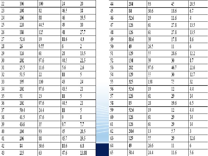
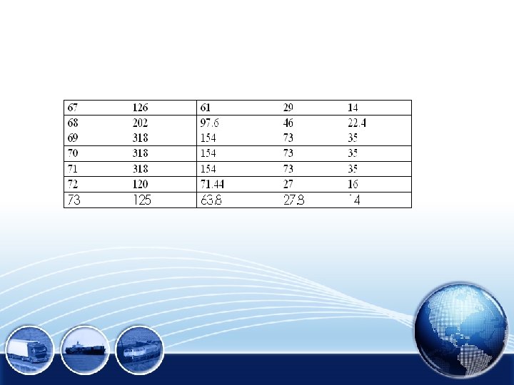
2. 2 Elements Of The Network : • number of Transformers : 73 Δ/Υ (33/0. 4) KV distribution transformers. • And the table shows the number of each of them and the rated KVA 630 KVA and 400 KVA has tap changer without load= ± 5% :

• The conducters used in the network are ACSR (120 mm 2 & 95 mm 2 & 50 mm 2) • The under ground cable used in the network are XLPE Cu (95 mm 2 & 50 mm 2)

2. 3 Electrical Consumption • The table below shows the total consumption of energy for 5 years. :

The daily load curve : We take readings to the load changes during the day, the result gives the graph below : The daily load curve we have very important information like: Max demand Load factor The suitable distribution of the load Total energy consumption How to avoid penalties and other important things

2. 4 Problems in The Network : • The P. F is less than 0. 92% , this cause penalties and power losses. • There is a voltage drop. • There is power losses.

3 Load Flow Analysis : *Apparent Power Measuring *Power factor and load factor calculations

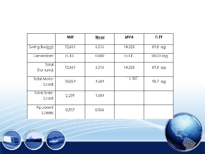
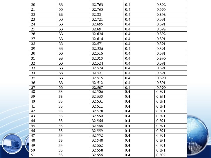
• By using etap power station we starting the study with the original case after the applying the data needed • like power factor and load consumption of power and other data : • The resultant basic information for TUBAS network with out connected the well came as shown in the following table:

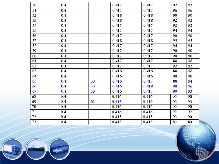
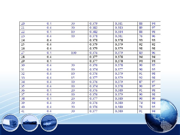
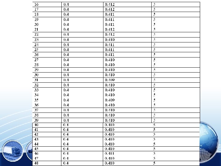
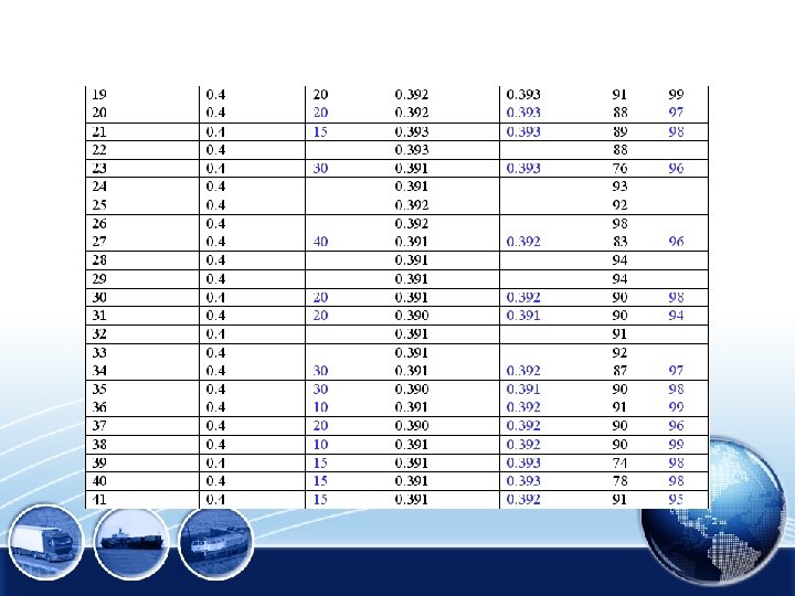
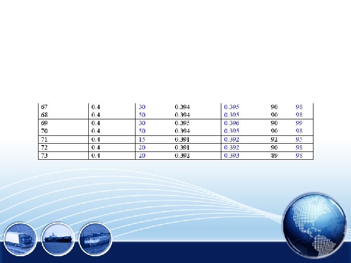
• The maximum case • 3. 1 the medium voltages & The low tension voltages • The actual medium voltages and low voltage on each transformer is shown in the table below :

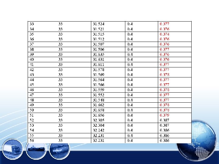

Note : the colored values refers to the least low voltages which has more drop of voltages.
")
• Value of maximum loads in table below: (before improvement)
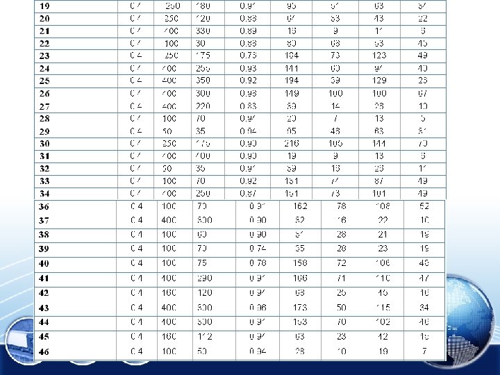


Note : the power factor less than 92%. This causes more penalties on the total bill

• SUMMARY • we have to summarize the results, total generation, demand , loading. , percentage of losses, and the total power factor The swing current = 240 A The p. f in the network equal 88. 3

• The maximum load improvement • we have # of methods in order to improve the network for a lot of positive effects such as reducing the cost / kwh. these methods are: • 1 - increasing the swing bus voltage • 2 - tab changing in the transformer. • 3 - adding capacitors to produce reactive power • 4 - change the connection of the network

increasing the swing bus voltage • In the network the connection point have the flexibility to increase the voltage on the swing bus up to 5% from the original voltage (33 kv) the new value of the swing bus voltage equal (34. 65 KV) the run of etab after applying this improvement the data shown in the following table:

• This table shows the bus voltage after increasing the swing bus voltage. • But we can't apply this method because the control of swing bus only by IEC

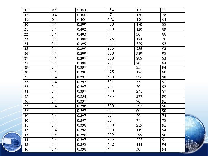
• improvement the max. case using tap changing • In this method of tab changing involves changing the tab ratio on the transformer but in limiting rang which not accede (5% ). • And after we applying this method we have the following result as shown In the table below : in


• This table show that the volteges of buses after improvement by changing the taps of transformer. The swing current = 258 A
- tan")
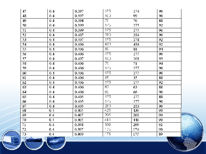
• Power factor improvement • Qc = P(tan cos (p. f old)- tan cos (p. f new)) = 957 KVAR • PF new at least = 92% , PF old = 89. 5 • The table below shows the voltage level before and after adding the capacitance:

• The result of basic information of the network after adding capacitance: The swing current = 251 A Origin Cace 258 A We note: and the total current decrease. Losses before p. f improvement = 0. 485 Mw. Losses after p. f improvement = 0. 460 Mw.

• the voltage level improvement using capacitors


• The result of basic information of the network after adding capacitance:

• • 5 Comparison between three case 1. the origin case. 2. power factor improvement case. 3. improvement using tap.


• • Minimum case : Value of minimum loads in table below: (before improvement)


• The medium & low tension voltages

The power factor on some transformers is low and we aim to rise both the power factor more than 0. 92 and voltages to reach 100% nearly.

• summary • we have to summarize the results, total generation, demand , loading. , percentage of losses, and the total power factor. The swing current = 95 A

• The minimum load improvement • The minimum case after improvement using tap


• we have to summarize the results, total generation, demand , loading. , percentage of losses, and the total power factor. The swing current = 99 A

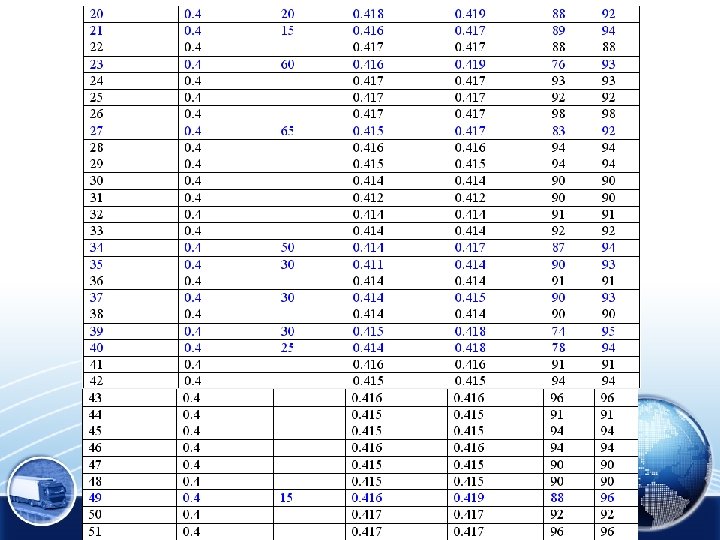
• Power factor improvement : • PF old = 90. 3 , PF new at least = 92% • Q=255 KVAR • The capacitor is added in delta connection parallel to the transformer in secondary side(0. 4 kv). • The table below shows the voltage level before and after adding the capacitance:


Total capacitors = 250 kvar

• we have to summarize the results, total generation, demand , loading. , percentage of losses, and the total power factor. The swing current = 97 A Orgin current = 99 A Losses before p. f improvement = 0. 072 Mw. Losses after p. f improvement = 0. 069 Mw.

• Comparison between three case • 1. the origin case. • 2. power factor improvement case. • 3. improvement using tap changing.


• voltage level improvement using capacitors:


• The result of basic information of the network after adding capacitance:

• Two connection point • SUMMARY OF TOTAL GENERATION, LOADING & DEMAND

• Comparison between two case • 1. one connection point • 2. two connection point


We notes Losses before = 0. 421 MW Losses after =0. 387 MW

• Economical Study • _Pmax=13. 215 mw • • • _Pmin=5. 126 mw _Losses before improvement =0. 485 mw _Losses after improvement =0. 46 mw _(Pf )before improvement in max. case=0. 895 _(Pf) before imrovement in min. case=0. 905 _(Pf) after improvement=0. 92 • To find the economical operation of the network we must do the following calculation: • • • Pav=(Pmax+Pmin)/2=(13. 215+5. 126)/2=9. 1705 mw LF=Pav/Pmax=0. 7 Total energy per year=Pmax*LF*total hour per year =13. 215*0. 7*8760=80333. 58*10^3 KWH Total cost per year=total energy*cost(NIS/KWH) =80333. 58*10^3*0. 33=26510. 08*10^3 NIS/YEAR
: Table below show relation of PF to")
• Saving in penalties of( PF): Table below show relation of PF to the penalties : Penalties=0. 01*(0. 92 -pf)*total bill =0. 01*0. 02*26510. 08*10^3=5300 NIS/YEAR

• Cost of losses : • • • • Losses before improvement=0. 485*0. 7=339. 5 kw Energy=339. 5*8760=2974. 02*10^3 kwh Total cost=2974. 02*10^3*0. 33=981426 NIS/YEAR Losses after improvement=460*0. 7=322 kw Energy=2820. 72 kwh Cost of losses=2820. 72*0. 33=930837 NIS/YEAR Saving in cost of losses=cost before improvement-cost after improvement =50859 NIS/YEAR Total capacitor =957 kvar (Cost per KVAR)with control circuit=15 JD=75 NIS Total cost of capacitors=957*75=71775 NIS Total saving=saving in penalties+ saving in losses =5300+50589=55889 • • S. P. B. P=(investment)/(saving) =71775/55889=1. 28 YEAR.
f2bae6bf5463b95d064019dcb97c294d.ppt