Trade Scheduling in Equity Markets Theory and Practice

Trade Scheduling in Equity Markets: Theory and Practice Michael Simmonds Liquid Markets Analytics STRICTLY PRIVATE AND CONFIDENTIAL © Nomura International plc

Section Header (used to create Tab Pages and Table of Contents) Contents n Nomura (Company and Analytics Teams) n Trade Scheduling Framework n Transaction Cost Estimation n Liquidity Prediction n Risk Estimation n Trade Scheduling Optimisation n Applications Source: 1

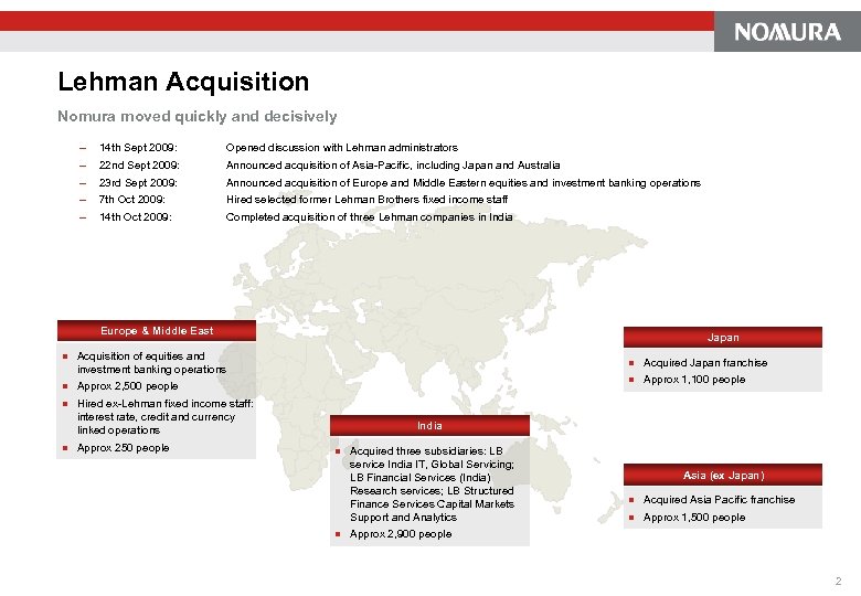Lehman Acquisition Nomura moved quickly and decisively - 14 th Sept 2009: Opened discussion with Lehman administrators 22 nd Sept 2009: Announced acquisition of Asia-Pacific, including Japan and Australia 23 rd Sept 2009: Announced acquisition of Europe and Middle Eastern equities and investment banking operations 7 th Oct 2009: Hired selected former Lehman Brothers fixed income staff 14 th Oct 2009: Completed acquisition of three Lehman companies in India Europe & Middle East n Acquisition of equities and investment banking operations n Approx 2, 500 people n Japan Hired ex-Lehman fixed income staff: interest rate, credit and currency linked operations n Approx 250 people n Acquired Japan franchise n Approx 1, 100 people India n n Acquired three subsidiaries: LB service India IT, Global Servicing; LB Financial Services (India) Research services; LB Structured Finance Services Capital Markets Support and Analytics Asia (ex Japan) n Acquired Asia Pacific franchise n Approx 1, 500 people Approx 2, 900 people 2

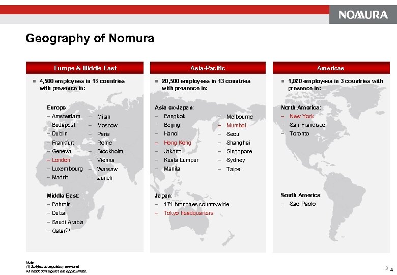Geography of Nomura Europe & Middle East n 4, 500 employees in 18 countries with presence in: Europe: – – – – Amsterdam – Budapest – Dublin – Frankfurt – Geneva – London – Luxembourg – Madrid – Asia-Pacific n Americas 20, 500 employees in 13 countries with presence in: Asia ex-Japan: Milan Moscow Paris Rome Stockholm Vienna Warsaw – – – – Bangkok Beijing Hanoi Hong Kong Jakarta Kuala Lumpur Manila n 1, 060 employees in 3 countries with presence in: North America: – – – – Melbourne Mumbai Seoul – New York – San Francisco – Toronto Shanghai Singapore Sydney Taipei Zurich Middle East: Japan: South America: – – – 171 branches countrywide – Tokyo headquarters – Sao Paolo Bahrain Dubai Saudi Arabia Qatar(1) Note: (1) Subject to regulatory approval. All headcount figures are approximate. 3 4

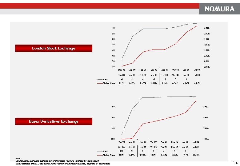London Stock Exchange Eurex Derivatives Exchange Note: London Stock Exchange statistics are whole trading volumes, weighted by value traded Eurex statistics are for Listed Equity Index Volume whole traded volumes, weighted by value traded 4 5

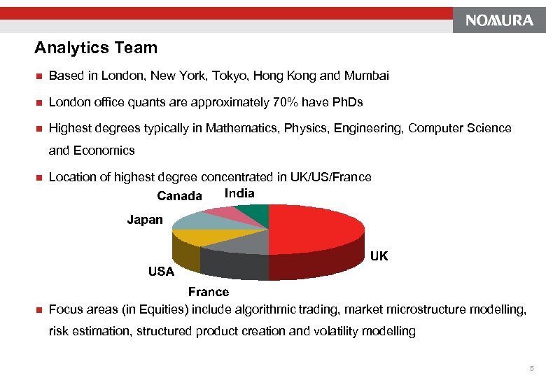Section Header (used to create Tab Pages and Table of Contents) Analytics Team n Based in London, New York, Tokyo, Hong Kong and Mumbai n London office quants are approximately 70% have Ph. Ds n Highest degrees typically in Mathematics, Physics, Engineering, Computer Science and Economics n Location of highest degree concentrated in UK/US/France n Focus areas (in Equities) include algorithmic trading, market microstructure modelling, risk estimation, structured product creation and volatility modelling 5

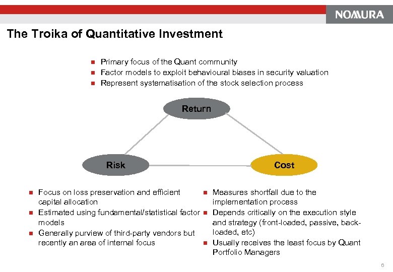The Troika of Quantitative Investment n n n Primary focus of the Quant community Factor models to exploit behavioural biases in security valuation Represent systematisation of the stock selection process Return Risk n n n Focus on loss preservation and efficient capital allocation Estimated using fundamental/statistical factor models Generally purview of third-party vendors but recently an area of internal focus Cost n n n Measures shortfall due to the implementation process Depends critically on the execution style and strategy (front-loaded, passive, backloaded, etc) Usually receives the least focus by Quant Portfolio Managers 6

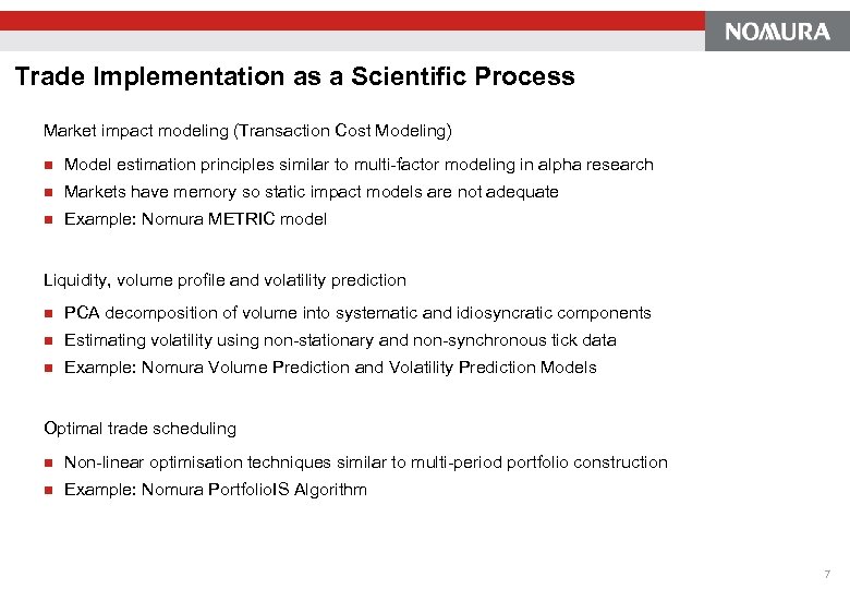Trade Implementation as a Scientific Process Market impact modeling (Transaction Cost Modeling) n Model estimation principles similar to multi-factor modeling in alpha research n Markets have memory so static impact models are not adequate n Example: Nomura METRIC model Liquidity, volume profile and volatility prediction n PCA decomposition of volume into systematic and idiosyncratic components n Estimating volatility using non-stationary and non-synchronous tick data n Example: Nomura Volume Prediction and Volatility Prediction Models Optimal trade scheduling n Non-linear optimisation techniques similar to multi-period portfolio construction n Example: Nomura Portfolio. IS Algorithm 7

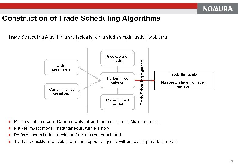Construction of Trade Scheduling Algorithms Price evolution model Order parameters Performance criterion Current market conditions Market impact model Trade Scheduling Algorithms are typically formulated as optimisation problems Trade Schedule: Number of shares to trade in each bin n Price evolution model: Random walk, Short-term momentum, Mean-reversion n Market impact model: Instantaneous, with Memory n Performance criteria – deviation from a target benchmark n Trade as quickly as possible to reduce opportunity cost without causing market impact 8

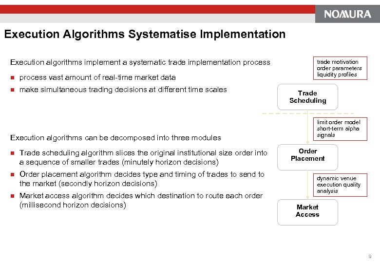Execution Algorithms Systematise Implementation Execution algorithms implement a systematic trade implementation process vast amount of real-time market data n make simultaneous trading decisions at different time scales Execution algorithms can be decomposed into three modules n Trade scheduling algorithm slices the original institutional size order into a sequence of smaller trades (minutely horizon decisions) n Order placement algorithm decides type and timing of trades to send to the market (secondly horizon decisions) n Market access algorithm decides which destination to route each order (millisecond horizon decisions) trade motivation order parameters liquidity profiles Trade Scheduling limit order model short-term alpha signals Order Placement dynamic venue execution quality analysis Market Access 9

10

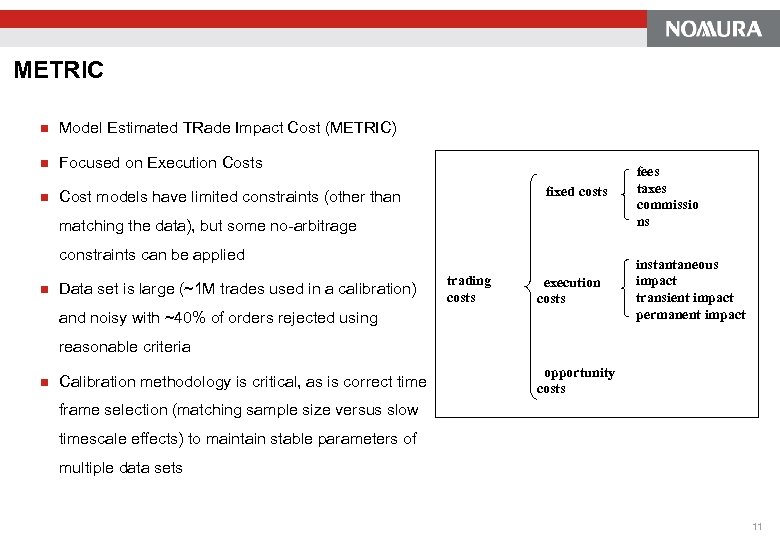METRIC n Model Estimated TRade Impact Cost (METRIC) n Focused on Execution Costs n Cost models have limited constraints (other than fixed costs matching the data), but some no-arbitrage constraints can be applied n Data set is large (~1 M trades used in a calibration) trading costs execution costs and noisy with ~40% of orders rejected using fees taxes commissio ns instantaneous impact transient impact permanent impact reasonable criteria n Calibration methodology is critical, as is correct time opportunity costs frame selection (matching sample size versus slow timescale effects) to maintain stable parameters of multiple data sets 11

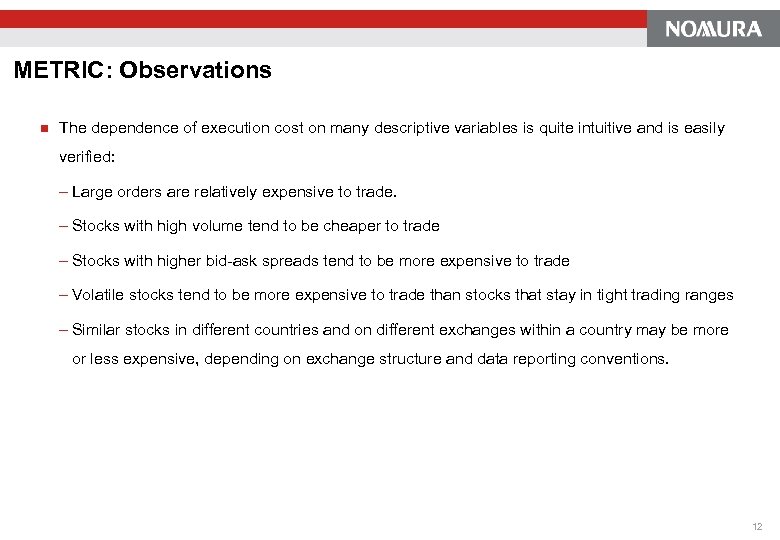METRIC: Observations n The dependence of execution cost on many descriptive variables is quite intuitive and is easily verified: - Large orders are relatively expensive to trade. - Stocks with high volume tend to be cheaper to trade - Stocks with higher bid-ask spreads tend to be more expensive to trade - Volatile stocks tend to be more expensive to trade than stocks that stay in tight trading ranges - Similar stocks in different countries and on different exchanges within a country may be more or less expensive, depending on exchange structure and data reporting conventions. 12

METRIC: Structure n Decompose cost into three parts: - Instantaneous impact: A measure of our micro execution skills which only affects child orders individually and then dissipates immediately. - Transient impact: Caused by temporary imbalances between supply and demand caused by our trades which lead to temporary price movement from equilibrium. Transient impact induced price will reverse after our trade and decay to 0 at the end. - Permanent impact: Impact due to changes in the equilibrium price caused by our trading, which accumulates and remains for the life of the trade. Permanent impact induced price will not mean reverse and stay at the end price level after trading. Therefore, we can capture permanent impact if and only if we wait long enough. 13

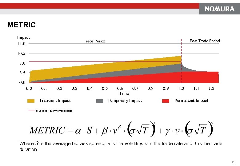METRIC Trade Period Post-Trade Period Total impact over the trade period Where S is the average bid-ask spread, is the volatility, v is the trade rate and T is the trade duration 14

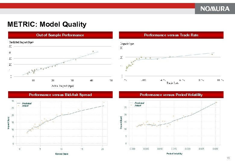METRIC: Model Quality Out of Sample Performance versus Trade Rate Performance versus Bid-Ask Spread Performance versus Period Volatility 15

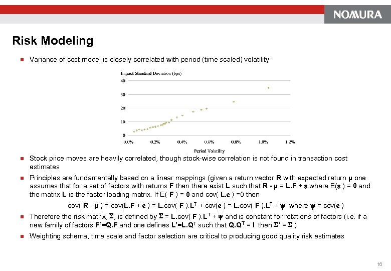Risk Modeling n Variance of cost model is closely correlated with period (time scaled) volatility n Stock price moves are heavily correlated, though stock-wise correlation is not found in transaction cost estimates n Principles are fundamentally based on a linear mappings (given a return vector R with expected return µ one assumes that for a set of factors with returns F then there exist L such that R - µ = L. F + where E( ) = 0 and the matrix L is the factor loading matrix. If E( F ) = 0 and cov( L. ) =0 then cov( R - µ ) = cov(L. F + ) = L. cov( F ). LT + cov( ) = L. cov( F ). LT + where = cov( ) n Therefore the risk matrix, , is defined by = L. cov( F ). LT + and is constant for rotations of factors (i. e. if a new family of factors F’=Q. F and one defines L’=L. QT such that Q. QT = I then ’ = ) n Weighting schema, time scale and factor selection are critical to producing good quality risk estimates 16

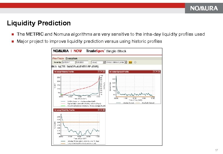Liquidity Prediction n The METRIC and Nomura algorithms are very sensitive to the intra-day liquidity profiles used n Major project to improve liquidity prediction versus using historic profiles 17

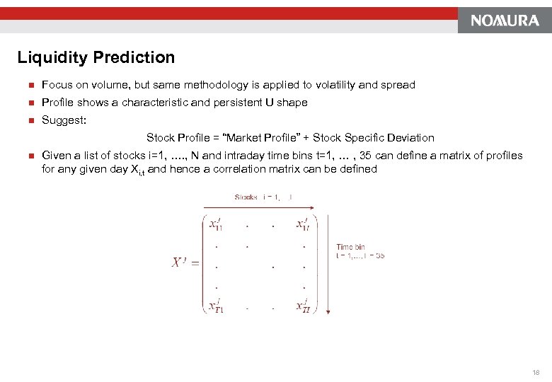Liquidity Prediction n Focus on volume, but same methodology is applied to volatility and spread n Profile shows a characteristic and persistent U shape n Suggest: Stock Profile = “Market Profile” + Stock Specific Deviation n Given a list of stocks i=1, …. , N and intraday time bins t=1, … , 35 can define a matrix of profiles for any given day Xi, t and hence a correlation matrix can be defined 18

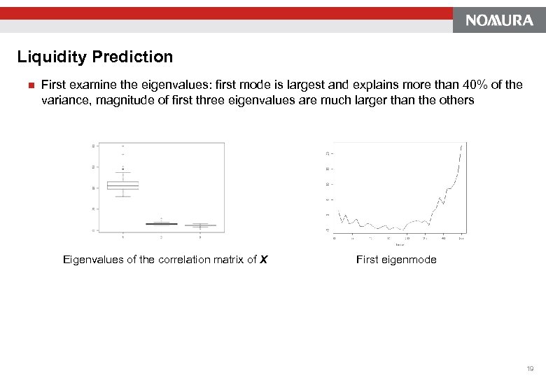Liquidity Prediction n First examine the eigenvalues: first mode is largest and explains more than 40% of the variance, magnitude of first three eigenvalues are much larger than the others Eigenvalues of the correlation matrix of X First eigenmode 19

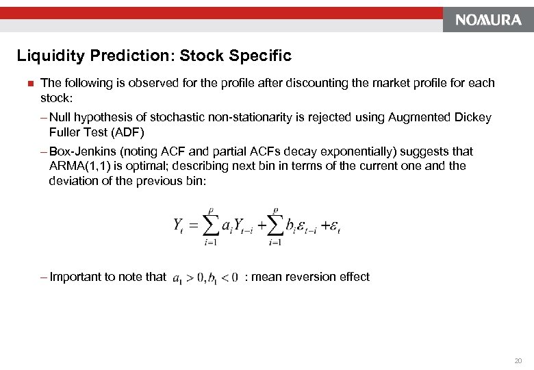Liquidity Prediction: Stock Specific n The following is observed for the profile after discounting the market profile for each stock: - Null hypothesis of stochastic non-stationarity is rejected using Augmented Dickey Fuller Test (ADF) - Box-Jenkins (noting ACF and partial ACFs decay exponentially) suggests that ARMA(1, 1) is optimal; describing next bin in terms of the current one and the deviation of the previous bin: - Important to note that : mean reversion effect 20

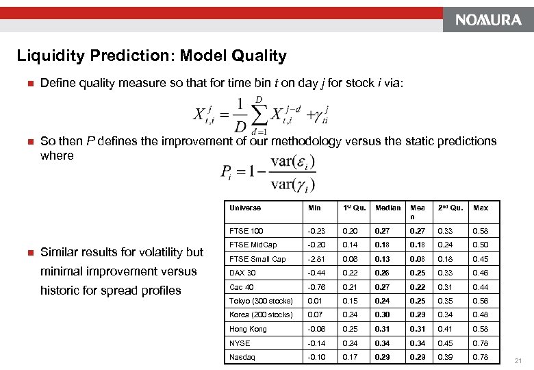Liquidity Prediction: Model Quality n Define quality measure so that for time bin t on day j for stock i via: n So then P defines the improvement of our methodology versus the static predictions where Universe 1 st Qu. Median Mea n 2 nd Qu. Max FTSE 100 n Min -0. 23 0. 20 0. 27 0. 33 0. 58 FTSE Mid. Cap -0. 20 0. 14 0. 18 0. 24 0. 50 FTSE Small Cap -2. 81 0. 06 0. 13 0. 08 0. 18 0. 45 minimal improvement versus DAX 30 -0. 44 0. 22 0. 26 0. 25 0. 33 0. 46 historic for spread profiles Cac 40 -0. 76 0. 21 0. 27 0. 22 0. 31 0. 44 Tokyo (300 stocks) 0. 01 0. 15 0. 24 0. 25 0. 35 0. 56 Korea (200 stocks) 0. 07 0. 24 0. 30 0. 29 0. 34 0. 48 Hong Kong -0. 06 0. 25 0. 31 0. 41 0. 58 NYSE -0. 14 0. 24 0. 34 0. 45 0. 78 Nasdaq -0. 10 0. 17 0. 29 0. 39 0. 78 Similar results for volatility but 21

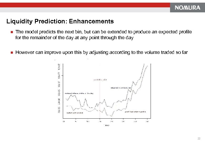Liquidity Prediction: Enhancements n The model predicts the next bin, but can be extended to produce an expected profile for the remainder of the day at any point through the day n However can improve upon this by adjusting according to the volume traded so far 22

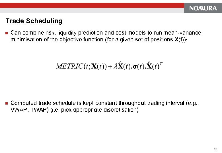Trade Scheduling n Can combine risk, liquidity prediction and cost models to run mean-variance minimisation of the objective function (for a given set of positions X(t)): n Computed trade schedule is kept constant throughout trading interval (e. g. , VWAP, TWAP) (i. e. pick appropriate discretisation) 23

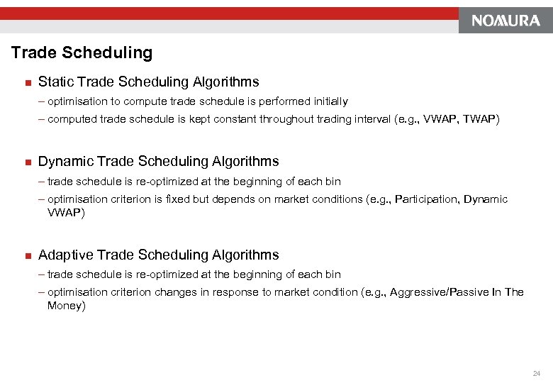Trade Scheduling n Static Trade Scheduling Algorithms - optimisation to compute trade schedule is performed initially - computed trade schedule is kept constant throughout trading interval (e. g. , VWAP, TWAP) n Dynamic Trade Scheduling Algorithms - trade schedule is re-optimized at the beginning of each bin - optimisation criterion is fixed but depends on market conditions (e. g. , Participation, Dynamic VWAP) n Adaptive Trade Scheduling Algorithms - trade schedule is re-optimized at the beginning of each bin - optimisation criterion changes in response to market condition (e. g. , Aggressive/Passive In The Money) 24

Conclusions n Cash markets require a variety of different modeling techniques to trade effectively n Calibration methodology is critical to maintain stable and explanatory models n Trade data and intraday data are both critical to effective trade scheduling n Most clients of top-tier brokers have insufficient data (and possibly quantitative resources) to manage this process themselves n Second tier brokers will struggle to keep pace with developments and may be forced to “white label” algorithms 25

References n Almgren, Chriss, “Optimal Execution of Portfolio Transactions” (2001) n Almgren, Lorenz, “Adaptive Arrival Price” (2006) n Bialkowski, Darolles and Le Fol, “Decomposing Volume for VWAP Strategies” (2005) 26