Topics Related to Data Mining CS 4 59995

Topics Related to Data Mining CS 4/59995

Information Retrieval • • • Relevance Ranking Using Terms Relevance Using Hyperlinks Synonyms. , Homonyms, and Ontologies Indexing of Documents Measuring Retrieval Effectiveness Information Retrieval and Structured Data

Information Retrieval Systems • Information retrieval (IR) systems use a simpler data model than database systems – Information organized as a collection of documents – Documents are unstructured, no schema • Information retrieval locates relevant documents, on the basis of user input such as keywords or example documents – e. g. , find documents containing the words “database systems” • Can be used even on textual descriptions provided with nontextual data such as images

Keyword Search • In full text retrieval, all the words in each document are considered to be keywords. – We use the word term to refer to the words in a document • Information-retrieval systems typically allow query expressions formed using keywords and the logical connectives and, or, and not – Ands are implicit, even if not explicitly specified • Ranking of documents on the basis of estimated relevance to a query is critical – Relevance ranking is based on factors such as • Term frequency – Frequency of occurrence of query keyword in document • Inverse document frequency – How many documents the query keyword occurs in » Fewer give more importance to keyword • Hyperlinks to documents – More links to a document is more important

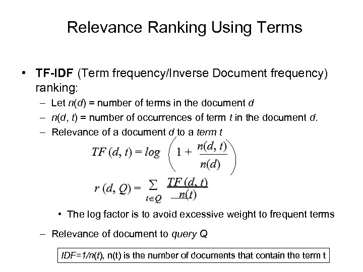Relevance Ranking Using Terms • TF-IDF (Term frequency/Inverse Document frequency) ranking: – Let n(d) = number of terms in the document d – n(d, t) = number of occurrences of term t in the document d. – Relevance of a document d to a term t 1 + n(d, t) n(d) r (d, Q) = TFn(d), t) (t t Q TF (d, t) = log • The log factor is to avoid excessive weight to frequent terms – Relevance of document to query Q IDF=1/n(t), n(t) is the number of documents that contain the term t

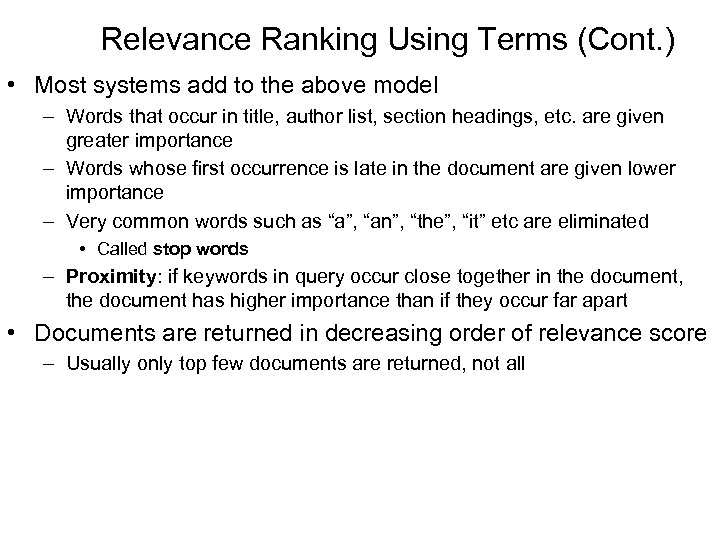Relevance Ranking Using Terms (Cont. ) • Most systems add to the above model – Words that occur in title, author list, section headings, etc. are given greater importance – Words whose first occurrence is late in the document are given lower importance – Very common words such as “a”, “an”, “the”, “it” etc are eliminated • Called stop words – Proximity: if keywords in query occur close together in the document, the document has higher importance than if they occur far apart • Documents are returned in decreasing order of relevance score – Usually only top few documents are returned, not all

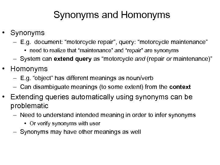Synonyms and Homonyms • Synonyms – E. g. document: “motorcycle repair”, query: “motorcycle maintenance” • need to realize that “maintenance” and “repair” are synonyms – System can extend query as “motorcycle and (repair or maintenance)” • Homonyms – E. g. “object” has different meanings as noun/verb – Can disambiguate meanings (to some extent) from the context • Extending queries automatically using synonyms can be problematic – Need to understand intended meaning in order to infer synonyms • Or verify synonyms with user – Synonyms may have other meanings as well

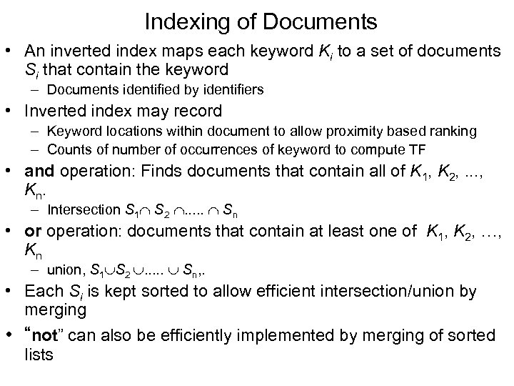Indexing of Documents • An inverted index maps each keyword Ki to a set of documents Si that contain the keyword – Documents identified by identifiers • Inverted index may record – Keyword locations within document to allow proximity based ranking – Counts of number of occurrences of keyword to compute TF • and operation: Finds documents that contain all of K 1, K 2, . . . , K n. – Intersection S 1 S 2 . . . Sn • or operation: documents that contain at least one of K 1, K 2, …, Kn – union, S 1 S 2 . . . Sn, . • Each Si is kept sorted to allow efficient intersection/union by merging • “not” can also be efficiently implemented by merging of sorted lists

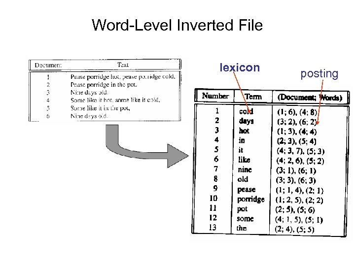Word-Level Inverted File lexicon posting

Measuring Retrieval Effectiveness • Information-retrieval systems save space by using index structures that support only approximate retrieval. May result in: – false negative (false drop) - some relevant documents may not be retrieved. – false positive - some irrelevant documents may be retrieved. – For many applications a good index should not permit any false drops, but may permit a few false positives. • Relevant performance metrics: – precision - what percentage of the retrieved documents are relevant to the query. – recall - what percentage of the documents relevant to the query were retrieved.

Measuring Retrieval Effectiveness (Cont. ) • Recall vs. precision tradeoff: • Can increase recall by retrieving many documents (down to a low level of relevance ranking), but many irrelevant documents would be fetched, reducing precision • Measures of retrieval effectiveness: – Recall as a function of number of documents fetched, or – Precision as a function of recall – Equivalently, as a function of number of documents fetched – E. g. “precision of 75% at recall of 50%, and 60% at a recall of 75%” • Problem: which documents are actually relevant, and which are not

Information Retrieval and Structured Data • Information retrieval systems originally treated documents as a collection of words • Information extraction systems infer structure from documents, e. g. : – Extraction of house attributes (size, address, number of bedrooms, etc. ) from a text advertisement – Extraction of topic and people named from a new article • Relations or XML structures used to store extracted data – System seeks connections among data to answer queries – Question answering systems

Probabilities and Statistic

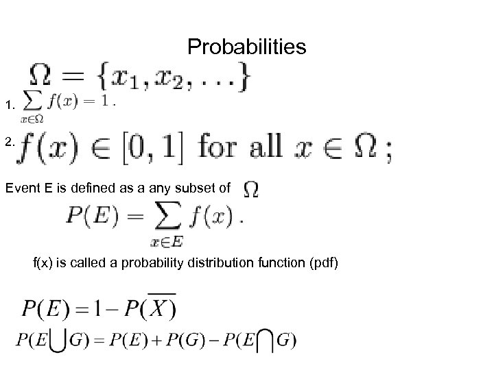Probabilities 1. 2. Event E is defined as a any subset of f(x) is called a probability distribution function (pdf)

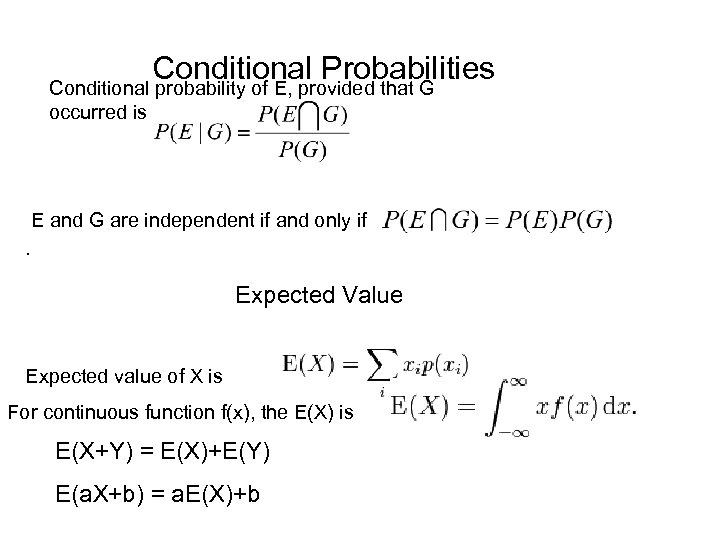Conditional Probabilities Conditional probability of E, provided that G occurred is E and G are independent if and only if. Expected Value Expected value of X is For continuous function f(x), the E(X) is E(X+Y) = E(X)+E(Y) E(a. X+b) = a. E(X)+b

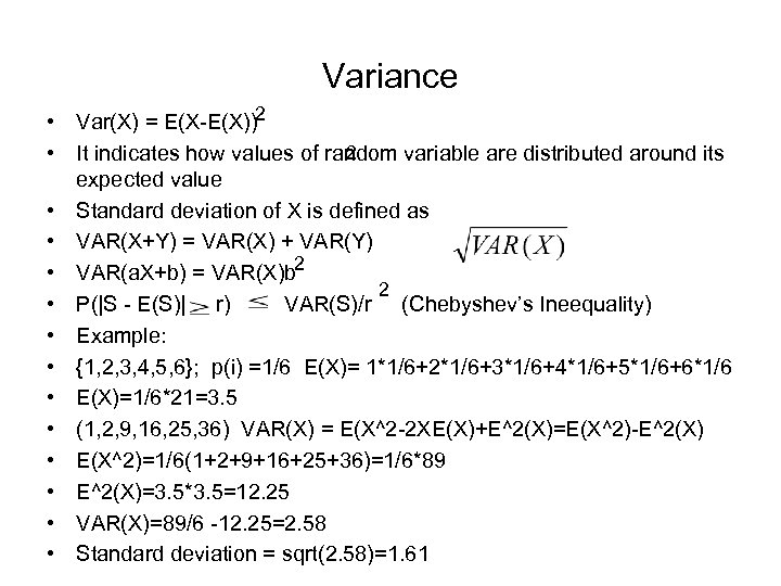Variance • Var(X) = E(X-E(X))2 2 • It indicates how values of random variable are distributed around its expected value • Standard deviation of X is defined as • VAR(X+Y) = VAR(X) + VAR(Y) • VAR(a. X+b) = VAR(X)b 2 2 • P(|S - E(S)| r) VAR(S)/r (Chebyshev’s Ineequality) • Example: • {1, 2, 3, 4, 5, 6}; p(i) =1/6 E(X)= 1*1/6+2*1/6+3*1/6+4*1/6+5*1/6+6*1/6 • E(X)=1/6*21=3. 5 • (1, 2, 9, 16, 25, 36) VAR(X) = E(X^2 -2 XE(X)+E^2(X)=E(X^2)-E^2(X) • E(X^2)=1/6(1+2+9+16+25+36)=1/6*89 • E^2(X)=3. 5*3. 5=12. 25 • VAR(X)=89/6 -12. 25=2. 58 • Standard deviation = sqrt(2. 58)=1. 61

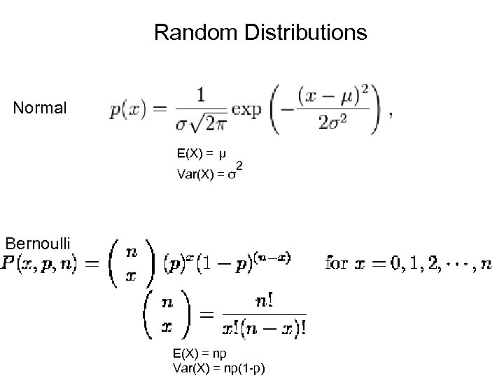Random Distributions Normal E(X) = μ Var(X) = σ 2 Bernoulli E(X) = np Var(X) = np(1 -p)

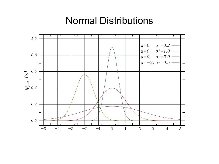Normal Distributions E(x) =

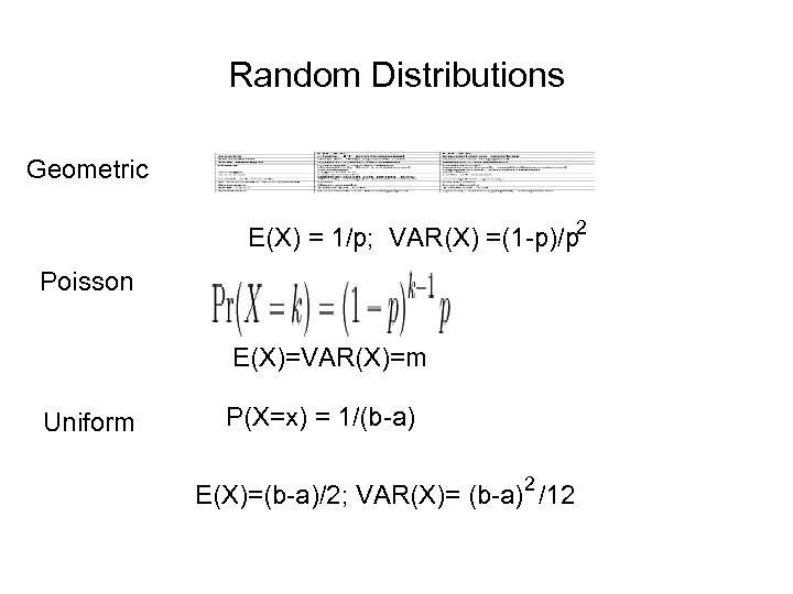Random Distributions Geometric E(X) = 1/p; VAR(X) =(1 -p)/p 2 Poisson E(X)=VAR(X)=m Uniform P(X=x) = 1/(b-a) E(X)=(b-a)/2; VAR(X)= (b-a)2 /12

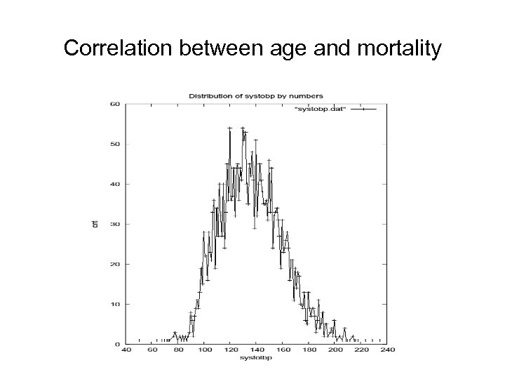Correlation between age and mortality

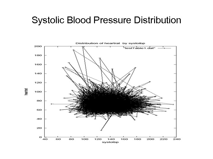Systolic Blood Pressure Distribution

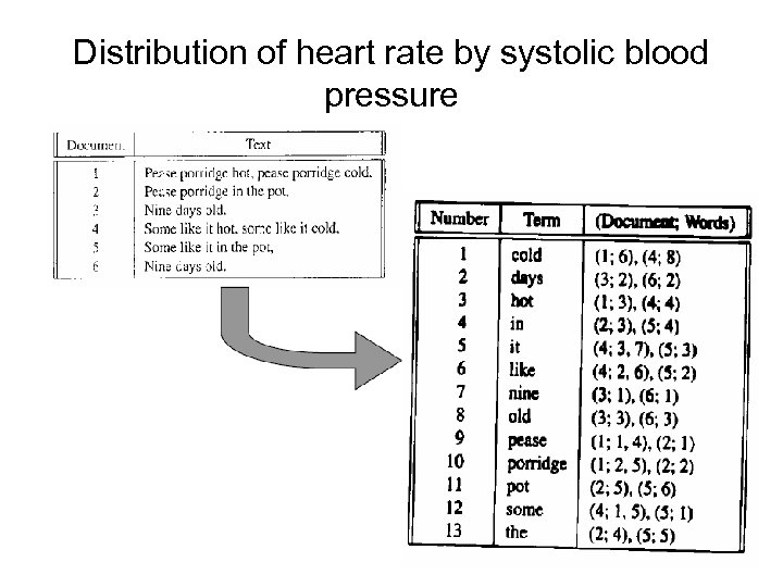Distribution of heart rate by systolic blood pressure

Data and their characteristics

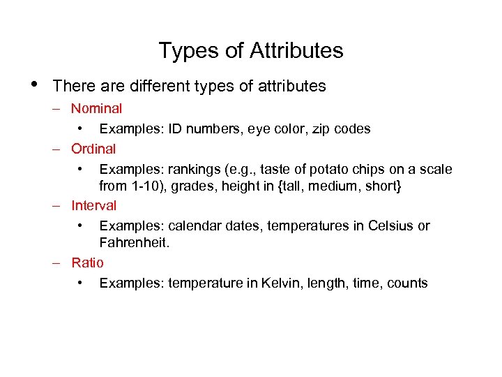Types of Attributes • There are different types of attributes – Nominal • Examples: ID numbers, eye color, zip codes – Ordinal • Examples: rankings (e. g. , taste of potato chips on a scale from 1 -10), grades, height in {tall, medium, short} – Interval • Examples: calendar dates, temperatures in Celsius or Fahrenheit. – Ratio • Examples: temperature in Kelvin, length, time, counts

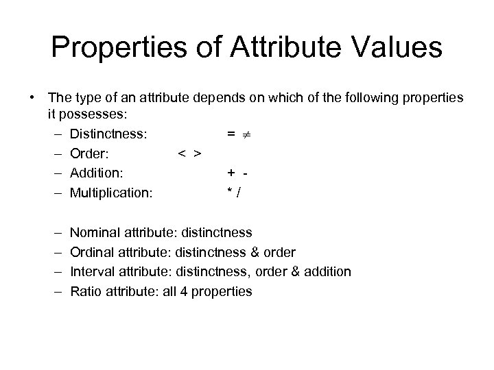Properties of Attribute Values • The type of an attribute depends on which of the following properties it possesses: – Distinctness: = – Order: < > – Addition: + – Multiplication: */ – – Nominal attribute: distinctness Ordinal attribute: distinctness & order Interval attribute: distinctness, order & addition Ratio attribute: all 4 properties

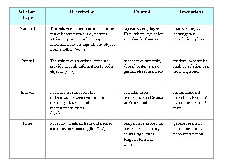Attribute Type Description Examples Nominal The values of a nominal attribute are just different names, i. e. , nominal attributes provide only enough information to distinguish one object from another. (=, ) zip codes, employee ID numbers, eye color, sex: {male, female} mode, entropy, contingency correlation, 2 test Ordinal The values of an ordinal attribute provide enough information to order objects. (<, >) hardness of minerals, {good, better, best}, grades, street numbers median, percentiles, rank correlation, run tests, sign tests Interval For interval attributes, the differences between values are meaningful, i. e. , a unit of measurement exists. (+, - ) calendar dates, temperature in Celsius or Fahrenheit mean, standard deviation, Pearson's correlation, t and F tests For ratio variables, both differences and ratios are meaningful. (*, /) temperature in Kelvin, monetary quantities, counts, age, mass, length, electrical current geometric mean, harmonic mean, percent variation Ratio Operations

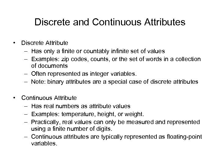Discrete and Continuous Attributes • Discrete Attribute – Has only a finite or countably infinite set of values – Examples: zip codes, counts, or the set of words in a collection of documents – Often represented as integer variables. – Note: binary attributes are a special case of discrete attributes • Continuous Attribute – Has real numbers as attribute values – Examples: temperature, height, or weight. – Practically, real values can only be measured and represented using a finite number of digits. – Continuous attributes are typically represented as floating-point variables.

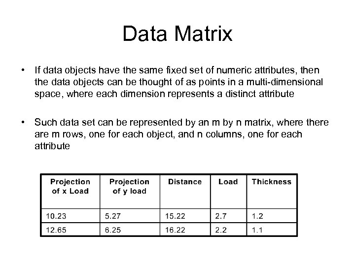Data Matrix • If data objects have the same fixed set of numeric attributes, then the data objects can be thought of as points in a multi-dimensional space, where each dimension represents a distinct attribute • Such data set can be represented by an m by n matrix, where there are m rows, one for each object, and n columns, one for each attribute

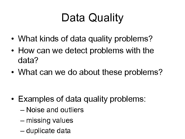Data Quality • What kinds of data quality problems? • How can we detect problems with the data? • What can we do about these problems? • Examples of data quality problems: – Noise and outliers – missing values – duplicate data

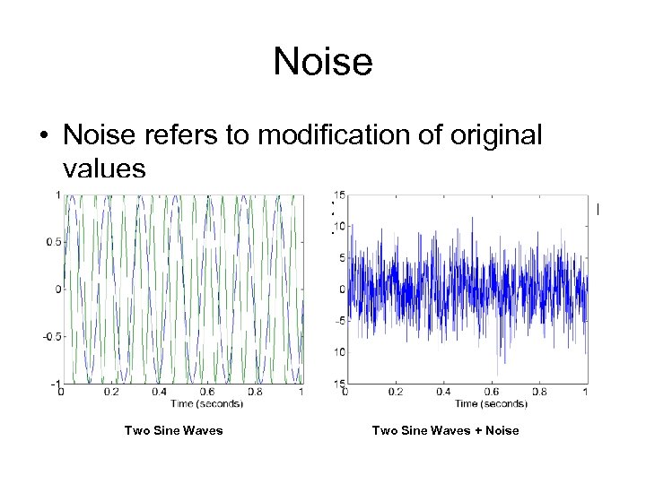Noise • Noise refers to modification of original values – Examples: distortion of a person’s voice when talking on a poor phone and “snow” on television screen Two Sine Waves + Noise

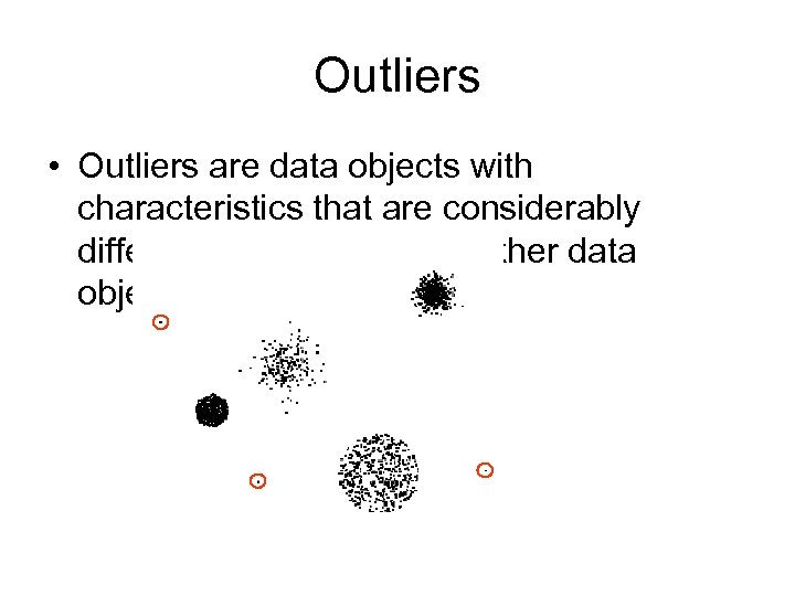Outliers • Outliers are data objects with characteristics that are considerably different than most of the other data objects in the data set

Data Preprocessing • • Aggregation Sampling Dimensionality Reduction Feature subset selection Feature creation Discretization and Binarization Attribute Transformation

Aggregation • Combining two or more attributes (or objects) into a single attribute (or object) • Purpose – Data reduction • Reduce the number of attributes or objects – Change of scale • Cities aggregated into regions, states, countries, etc – More “stable” data • Aggregated data tends to have less variability

Sampling • Sampling is the main technique employed for data selection. – It is often used for both the preliminary investigation of the data and the final data analysis. • Statisticians sample because obtaining the entire set of data of interest is too expensive or time consuming. • Sampling is used in data mining because processing the entire set of data of interest is too expensive or time consuming.

Sampling … • The key principle for effective sampling is the following: – using a sample will work almost as well as using the entire data sets, if the sample is representative – A sample is representative if it has approximately the same property (of interest) as the original set of data

Types of Sampling • Simple Random Sampling – There is an equal probability of selecting any particular item • Sampling without replacement – As each item is selected, it is removed from the population • Sampling with replacement – Objects are not removed from the population as they are selected for the sample. • In sampling with replacement, the same object can be picked up more than once • Stratified sampling – Split the data into several partitions; then draw random samples from each partition

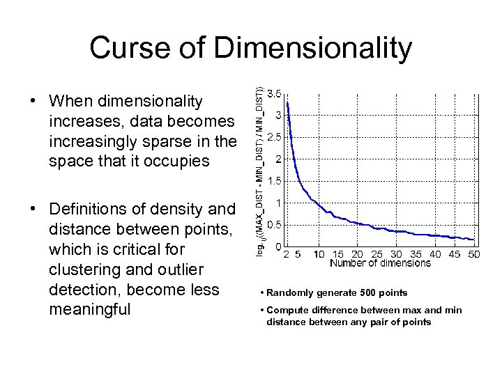Curse of Dimensionality • When dimensionality increases, data becomes increasingly sparse in the space that it occupies • Definitions of density and distance between points, which is critical for clustering and outlier detection, become less meaningful • Randomly generate 500 points • Compute difference between max and min distance between any pair of points

Discretization • Three types of attributes: – Nominal — values from an unordered set – Ordinal — values from an ordered set – Continuous — real numbers • Discretization: *divide the range of a continuous attribute into intervals – Some classification algorithms only accept categorical attributes. – Reduce data size by discretization – Prepare for further analysis

Discretization and Concept hierarchy • Discretization – reduce the number of values for a given continuous attribute by dividing the range of the attribute into intervals. Interval labels can then be used to replace actual data values. • Concept hierarchies – reduce the data by collecting and replacing low level concepts (such as numeric values for the attribute age) by higher level concepts (such as young, middle-aged, or senior).

Discretization • Three types of attributes: – Nominal — values from an unordered set – Ordinal — values from an ordered set – Continuous — real numbers • Discretization: *divide the range of a continuous attribute into intervals – Some classification algorithms only accept categorical attributes. – Reduce data size by discretization – Prepare for further analysis

Discretization and generation for numeric data • Binning • Histogram analysis • Entropy-based discretization • Segmentation by natural partitioning

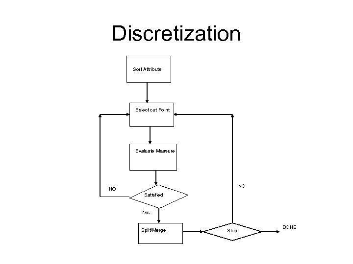Discretization Sort Attribute Select cut Point Evaluate Measure NO NO Satisfied Yes Split/Merge Stop DONE

Simple Discretization Methods: Binning • Equal-width (distance) partitioning: – It divides the range into N intervals of equal size: uniform grid – if A and B are the lowest and highest values of the attribute, the width of intervals will be: W = (B-A)/N. – The most straightforward – But outliers may dominate presentation – Skewed data is not handled well. • Equal-depth (frequency) partitioning: – It divides the range into N intervals, each containing approximately same number of samples – Good data scaling – Managing categorical attributes can be tricky.

Discretization • Three types of attributes: – Nominal — values from an unordered set – Ordinal — values from an ordered set – Continuous — real numbers • Discretization: *divide the range of a continuous attribute into intervals – Some classification algorithms only accept categorical attributes. – Reduce data size by discretization – Prepare for further analysis

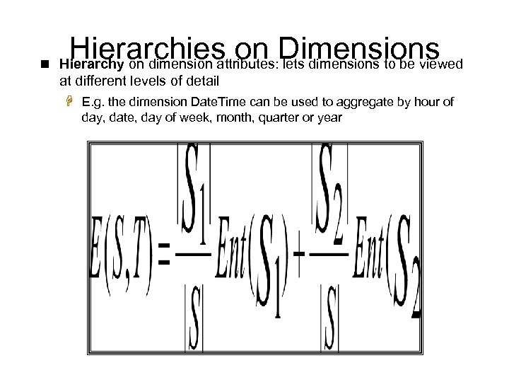
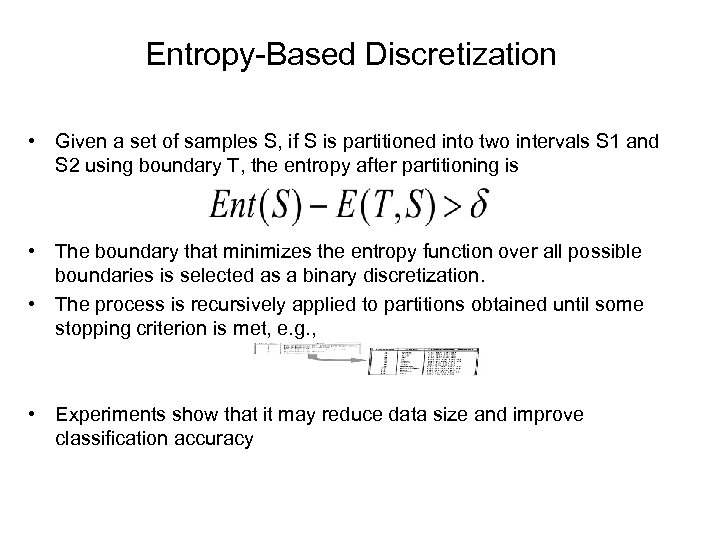Entropy-Based Discretization • Given a set of samples S, if S is partitioned into two intervals S 1 and S 2 using boundary T, the entropy after partitioning is • The boundary that minimizes the entropy function over all possible boundaries is selected as a binary discretization. • The process is recursively applied to partitions obtained until some stopping criterion is met, e. g. , • Experiments show that it may reduce data size and improve classification accuracy

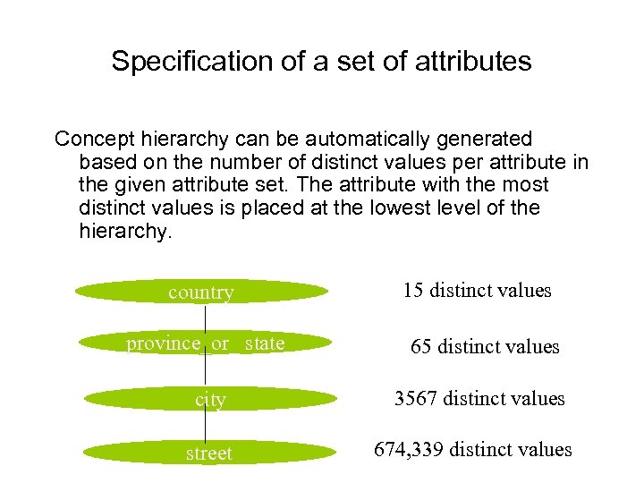Specification of a set of attributes Concept hierarchy can be automatically generated based on the number of distinct values per attribute in the given attribute set. The attribute with the most distinct values is placed at the lowest level of the hierarchy. country 15 distinct values province_or_ state 65 distinct values city 3567 distinct values street 674, 339 distinct values

Similarity and Dissimilarity • Similarity – Numerical measure of how alike two data objects are. – Is higher when objects are more alike. – Often falls in the range [0, 1] • Dissimilarity – Numerical measure of how different are two data objects – Lower when objects are more alike – Minimum dissimilarity is often 0 – Upper limit varies • Proximity refers to a similarity or dissimilarity

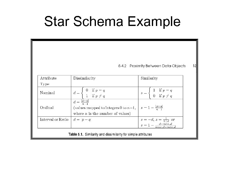
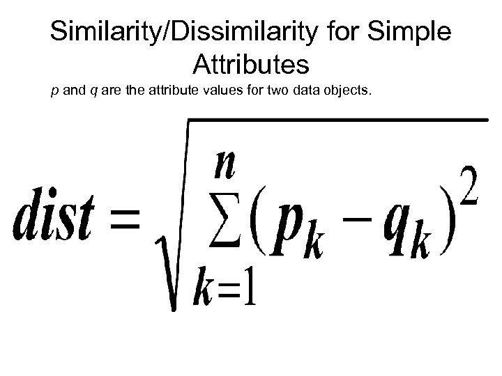Similarity/Dissimilarity for Simple Attributes p and q are the attribute values for two data objects.

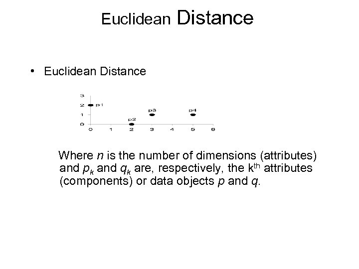Euclidean Distance • Euclidean Distance Where n is the number of dimensions (attributes) and pk and qk are, respectively, the kth attributes (components) or data objects p and q.

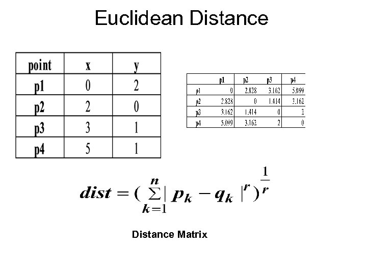Euclidean Distance Matrix

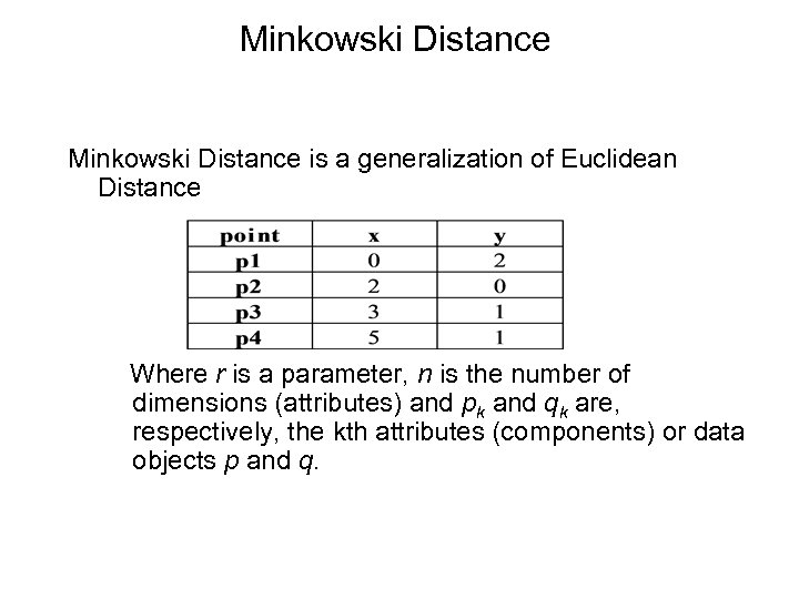Minkowski Distance is a generalization of Euclidean Distance Where r is a parameter, n is the number of dimensions (attributes) and pk and qk are, respectively, the kth attributes (components) or data objects p and q.

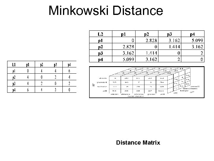Minkowski Distance Matrix

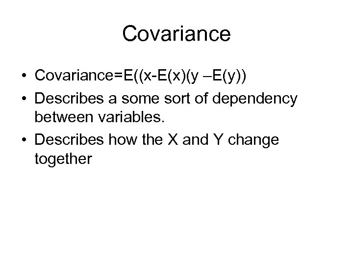Covariance • Covariance=E((x-E(x)(y –E(y)) • Describes a some sort of dependency between variables. • Describes how the X and Y change together

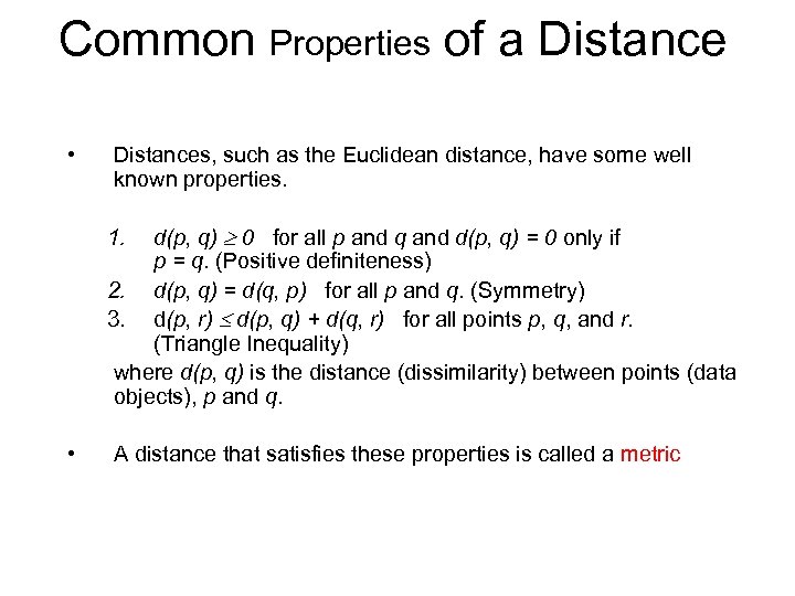Common Properties of a Distance • Distances, such as the Euclidean distance, have some well known properties. d(p, q) 0 for all p and q and d(p, q) = 0 only if p = q. (Positive definiteness) 2. d(p, q) = d(q, p) for all p and q. (Symmetry) 3. d(p, r) d(p, q) + d(q, r) for all points p, q, and r. (Triangle Inequality) where d(p, q) is the distance (dissimilarity) between points (data objects), p and q. 1. • A distance that satisfies these properties is called a metric

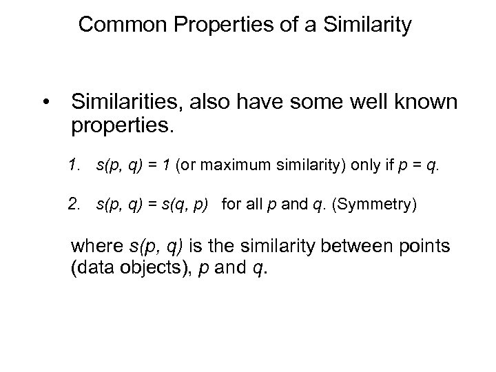Common Properties of a Similarity • Similarities, also have some well known properties. 1. s(p, q) = 1 (or maximum similarity) only if p = q. 2. s(p, q) = s(q, p) for all p and q. (Symmetry) where s(p, q) is the similarity between points (data objects), p and q.

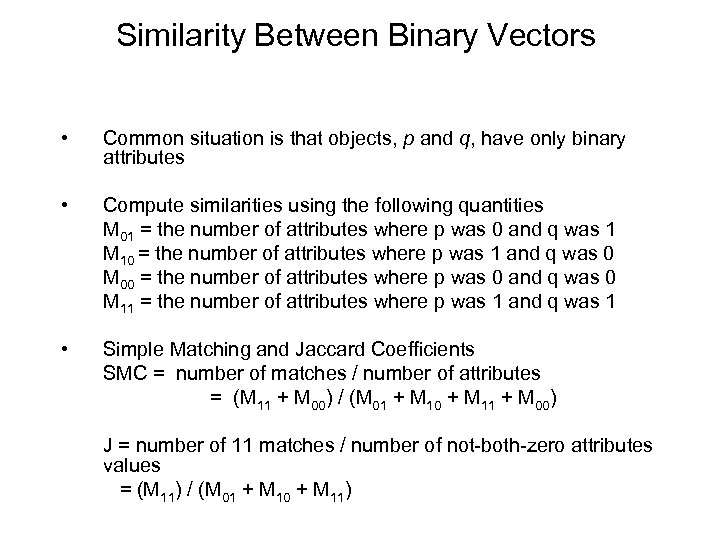Similarity Between Binary Vectors • Common situation is that objects, p and q, have only binary attributes • Compute similarities using the following quantities M 01 = the number of attributes where p was 0 and q was 1 M 10 = the number of attributes where p was 1 and q was 0 M 00 = the number of attributes where p was 0 and q was 0 M 11 = the number of attributes where p was 1 and q was 1 • Simple Matching and Jaccard Coefficients SMC = number of matches / number of attributes = (M 11 + M 00) / (M 01 + M 10 + M 11 + M 00) J = number of 11 matches / number of not-both-zero attributes values = (M 11) / (M 01 + M 10 + M 11)

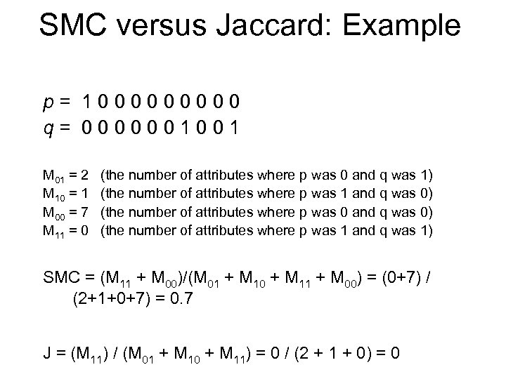SMC versus Jaccard: Example p= 100000 q= 0000001001 M 01 = 2 M 10 = 1 M 00 = 7 M 11 = 0 (the number of attributes where p was 0 and q was 1) (the number of attributes where p was 1 and q was 0) (the number of attributes where p was 0 and q was 0) (the number of attributes where p was 1 and q was 1) SMC = (M 11 + M 00)/(M 01 + M 10 + M 11 + M 00) = (0+7) / (2+1+0+7) = 0. 7 J = (M 11) / (M 01 + M 10 + M 11) = 0 / (2 + 1 + 0) = 0

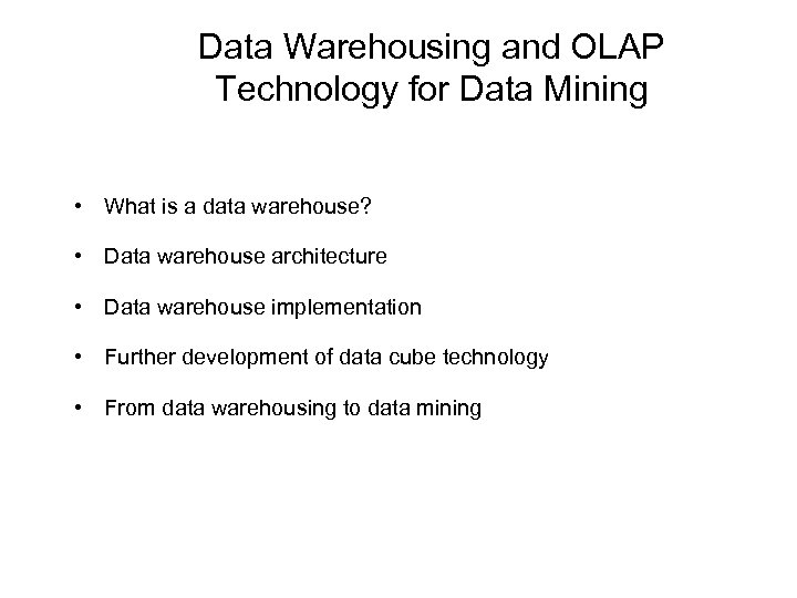Data Warehousing and OLAP Technology for Data Mining • What is a data warehouse? • Data warehouse architecture • Data warehouse implementation • Further development of data cube technology • From data warehousing to data mining

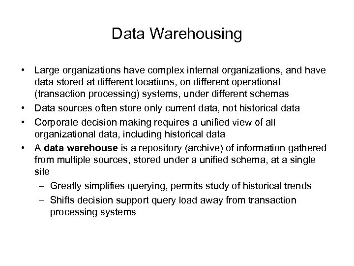Data Warehousing • Large organizations have complex internal organizations, and have data stored at different locations, on different operational (transaction processing) systems, under different schemas • Data sources often store only current data, not historical data • Corporate decision making requires a unified view of all organizational data, including historical data • A data warehouse is a repository (archive) of information gathered from multiple sources, stored under a unified schema, at a single site – Greatly simplifies querying, permits study of historical trends – Shifts decision support query load away from transaction processing systems

Data Warehouse vs. Operational DBMS • OLTP (on-line transaction processing) – Major task of traditional relational DBMS – Day-to-day operations: purchasing, inventory, banking, manufacturing, payroll, registration, accounting, etc. • OLAP (on-line analytical processing) – Major task of data warehouse system – Data analysis and decision making • Distinct features (OLTP vs. OLAP): – User and system orientation: customer vs. market – Data contents: current, detailed vs. historical, consolidated – Database design: ER + application vs. star + subject – View: current, local vs. evolutionary, integrated – Access patterns: update vs. read-only but complex queries

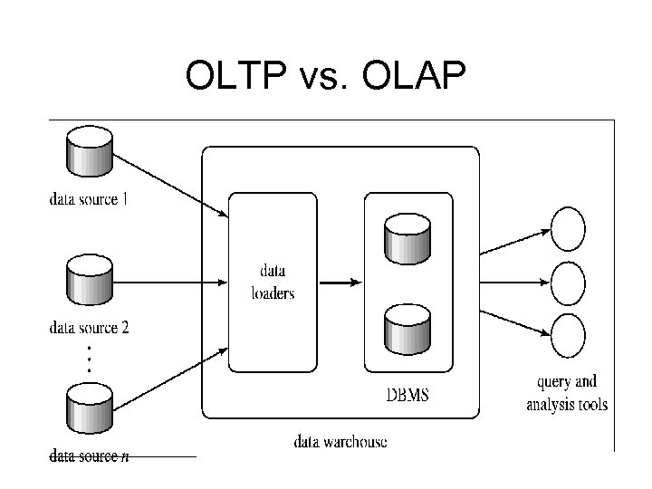OLTP vs. OLAP

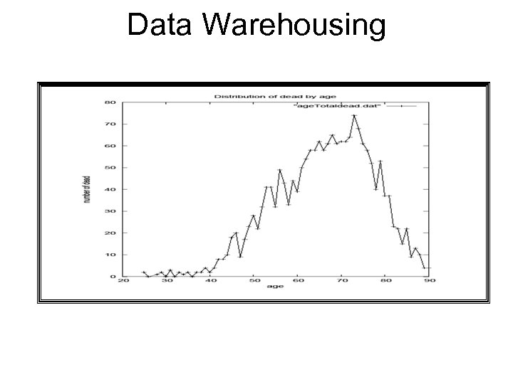Data Warehousing

Managing of a warehouse • When and how to gather data – Source driven architecture: data sources transmit new information to warehouse, either continuously or periodically (e. g. at night) – Destination driven architecture: warehouse periodically requests new information from data sources • What schema to use – Schema integration

Managing of a warehouse(Cont. ) • Data cleansing – E. g. correct mistakes in addresses • E. g. misspellings, zip code errors – Merge address lists from different sources and purge duplicates • Keep only one address record per household (“householding”) • How to propagate updates – Warehouse schema may be a (materialized) view of schema from data sources – Efficient techniques for update of materialized views • What data to summarize – Raw data may be too large to store on-line – Aggregate values (totals/subtotals) often suffice – Queries on raw data can often be transformed by query optimizer to use aggregate values

Conceptual Modeling of Data Warehouses • Modeling data warehouses: dimensions & measures – Star schema: A fact table in the middle connected to a set of dimension tables – Snowflake schema: A refinement of star schema where some dimensional hierarchy to snowflake – Fact constellations is normalized into a set of smaller dimension tables, forming a shape similar : Multiple fact tables share dimension tables, viewed as a collection of stars, therefore called galaxy schema or fact constellation

Star Schema Example

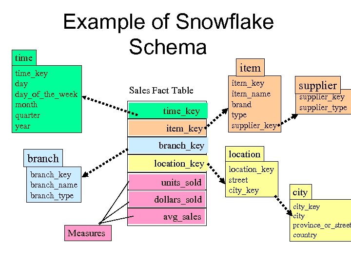time Example of Snowflake Schema time_key day_of_the_week month quarter year item Sales Fact Table time_key item_key branch location_key branch_name branch_type units_sold dollars_sold avg_sales Measures item_key item_name brand type supplier_key supplier_type location_key street city_key city province_or_street country

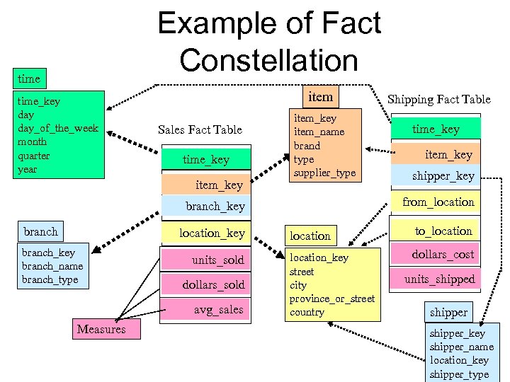Example of Fact Constellation time_key day_of_the_week month quarter year item Sales Fact Table time_key item_key item_name brand type supplier_type location_key branch_name branch_type units_sold dollars_sold avg_sales Measures time_key item_key shipper_key from_location branch_key branch Shipping Fact Table location to_location_key street city province_or_street country dollars_cost units_shipped shipper_key shipper_name location_key shipper_type

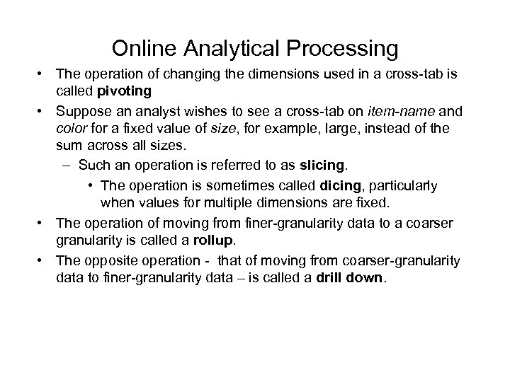Online Analytical Processing • The operation of changing the dimensions used in a cross-tab is called pivoting • Suppose an analyst wishes to see a cross-tab on item-name and color for a fixed value of size, for example, large, instead of the sum across all sizes. – Such an operation is referred to as slicing. • The operation is sometimes called dicing, particularly when values for multiple dimensions are fixed. • The operation of moving from finer-granularity data to a coarser granularity is called a rollup. • The opposite operation - that of moving from coarser-granularity data to finer-granularity data – is called a drill down.

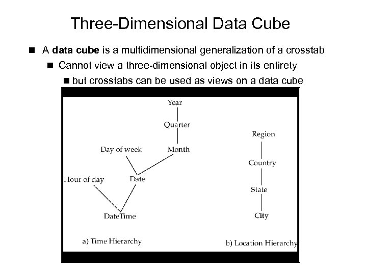Three-Dimensional Data Cube n A data cube is a multidimensional generalization of a crosstab n Cannot view a three-dimensional object in its entirety n but crosstabs can be used as views on a data cube

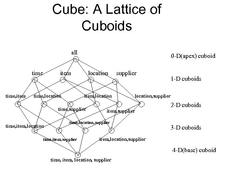Cube: A Lattice of Cuboids all time, item 0 -D(apex) cuboid item time, location item, location time, supplier time, item, location supplier location, supplier item, supplier time, location, supplier time, item, supplier 1 -D cuboids 2 -D cuboids 3 -D cuboids item, location, supplier 4 -D(base) cuboid time, item, location, supplier

Hierarchies on Dimensions n Hierarchy on dimension attributes: lets dimensions to be viewed at different levels of detail H E. g. the dimension Date. Time can be used to aggregate by hour of day, date, day of week, month, quarter or year

OLAP Implementation • The earliest OLAP systems used multidimensional arrays in memory to store data cubes, and are referred to as multidimensional OLAP (MOLAP) systems. • OLAP implementations using only relational database features are called relational OLAP (ROLAP) systems • Hybrid systems, which store some summaries in memory and store the base data and other summaries in a relational database, are called hybrid OLAP (HOLAP) systems.

OLAP Implementation (Cont. ) • Early OLAP systems precomputed all possible aggregates in order to provide online response – Space and time requirements for doing so can be very high • 2 n combinations of group by – It suffices to precompute some aggregates, and compute others on demand from one of the precomputed aggregates • Can compute aggregate on (item-name, color) from an aggregate on (item-name, color, size) – For all but a few “non-decomposable” aggregates such as median – is cheaper than computing it from scratch • Several optimizations available for computing multiple aggregates – Can compute aggregate on (item-name, color) from an aggregate on (item-name, color, size) – Can compute aggregates on (item-name, color, size), (item-name, color) and (item-name) using a single sorting of the base data

Group By cube • The cube operation computes union of group by’s on every subset of the specified attributes • E. g. consider the query select item-name, color, size, sum(number) from sales group by cube(item-name, color, size) This computes the union of eight different groupings of the sales relation: { (item-name, color, size), (item-name, color), (item-name, size), (color, size), (item-name), (color), (size), ()} where ( ) denotes an empty group by list. • For each grouping, the result contains the null value for attributes not present in the grouping.

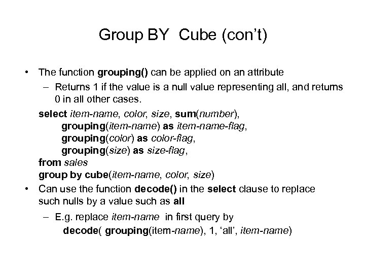Group BY Cube (con’t) • The function grouping() can be applied on an attribute – Returns 1 if the value is a null value representing all, and returns 0 in all other cases. select item-name, color, size, sum(number), grouping(item-name) as item-name-flag, grouping(color) as color-flag, grouping(size) as size-flag, from sales group by cube(item-name, color, size) • Can use the function decode() in the select clause to replace such nulls by a value such as all – E. g. replace item-name in first query by decode( grouping(item-name), 1, ‘all’, item-name)

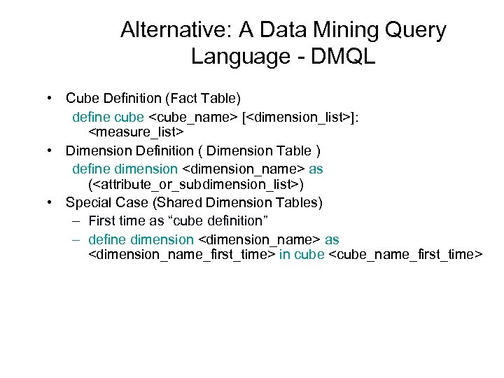Alternative: A Data Mining Query Language - DMQL • Cube Definition (Fact Table) define cube []: • Dimension Definition ( Dimension Table ) define dimension as () • Special Case (Shared Dimension Tables) – First time as “cube definition” – define dimension as in cube

Defining a Star Schema in DMQL define cube sales_star [time, item, branch, location]: dollars_sold = sum(sales_in_dollars), avg_sales = avg(sales_in_dollars), units_sold = count(*) define dimension time as (time_key, day_of_week, month, quarter, year) define dimension item as (item_key, item_name, brand, type, supplier_type) define dimension branch as (branch_key, branch_name, branch_type) define dimension location as (location_key, street, city, province_or_state, country)

Defining a Snowflake Schema in DMQL define cube sales_snowflake [time, item, branch, location]: dollars_sold = sum(sales_in_dollars), avg_sales = avg(sales_in_dollars), units_sold = count(*) define dimension time as (time_key, day_of_week, month, quarter, year) define dimension item as (item_key, item_name, brand, type, supplier(supplier_key, supplier_type)) define dimension branch as (branch_key, branch_name, branch_type) define dimension location as (location_key, street, city(city_key, province_or_state, country))

Defining a Fact Constellation in DMQL define cube sales [time, item, branch, location]: dollars_sold = sum(sales_in_dollars), avg_sales = avg(sales_in_dollars), units_sold = count(*) define dimension time as (time_key, day_of_week, month, quarter, year) define dimension item as (item_key, item_name, brand, type, supplier_type) define dimension branch as (branch_key, branch_name, branch_type) define dimension location as (location_key, street, city, province_or_state, country) define cube shipping [time, item, shipper, from_location, to_location]: dollar_cost = sum(cost_in_dollars), unit_shipped = count(*) define dimension time as time in cube sales define dimension item as item in cube sales define dimension shipper as (shipper_key, shipper_name, location as location in cube sales, shipper_type) define dimension from_location as location in cube sales define dimension to_location as location in cube sales

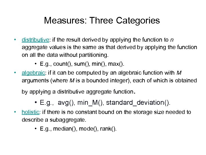Measures: Three Categories • distributive: if the result derived by applying the function to n aggregate values is the same as that derived by applying the function on all the data without partitioning. • E. g. , count(), sum(), min(), max(). • algebraic: if it can be computed by an algebraic function with M arguments (where M is a bounded integer), each of which is obtained by applying a distributive aggregate function . • E. g. , avg(), min_M(), standard_deviation(). • holistic: if there is no constant bound on the storage size needed to describe a subaggregate. • E. g. , median(), mode(), rank().

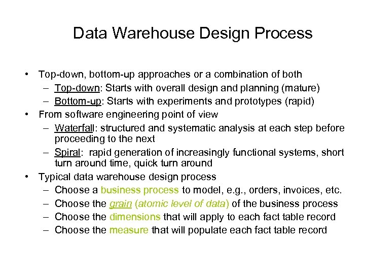Data Warehouse Design Process • Top-down, bottom-up approaches or a combination of both – Top-down: Starts with overall design and planning (mature) – Bottom-up: Starts with experiments and prototypes (rapid) • From software engineering point of view – Waterfall: structured and systematic analysis at each step before proceeding to the next – Spiral: rapid generation of increasingly functional systems, short turn around time, quick turn around • Typical data warehouse design process – Choose a business process to model, e. g. , orders, invoices, etc. – Choose the grain (atomic level of data) of the business process – Choose the dimensions that will apply to each fact table record – Choose the measure that will populate each fact table record

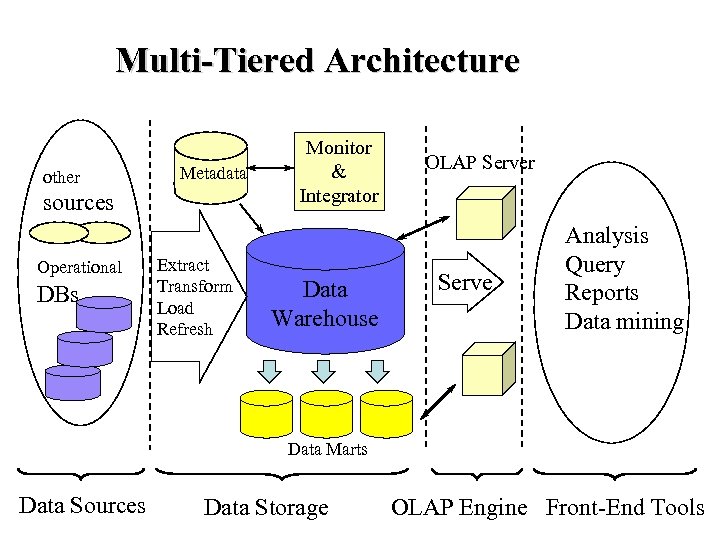Multi-Tiered Architecture other Metadata sources Operational DBs Extract Transform Load Refresh Monitor & Integrator Data Warehouse OLAP Server Serve Analysis Query Reports Data mining Data Marts Data Sources Data Storage OLAP Engine Front-End Tools

Efficient Processing OLAP Queries • Determine which operations should be performed on the available cuboids: – transform drill, roll, etc. into corresponding SQL and/or OLAP operations, e. g, dice = selection + projection • Determine to which materialized cuboid(s) the relevant operations should be applied. • Exploring indexing structures and compressed vs. dense array structures in MOLAP

Metadata Repository • Meta data is the data defining warehouse objects. It has the following kinds – Description of the structure of the warehouse • schema, view, dimensions, hierarchies, derived data defn, data mart locations and contents – Operational meta-data • data lineage (history of migrated data and transformation path), currency of data (active, archived, or purged), monitoring information (warehouse usage statistics, error reports, audit trails) – The algorithms used for summarization – The mapping from operational environment to the data warehouse – Data related to system performance • warehouse schema, view and derived data definitions – Business data • business terms and definitions, ownership of data, charging policies

Data Warehouse Back-End Tools and Utilities • Data extraction: – get data from multiple, heterogeneous, and external sources • Data cleaning: – detect errors in the data and rectify them when possible • Data transformation: – convert data from legacy or host format to warehouse format • Load: – sort, summarize, consolidate, compute views, check integrity, and build indicies and partitions • Refresh – propagate the updates from the data sources to the warehouse

Discovery-Driven Exploration of Data Cubes • Hypothesis-driven: exploration by user, huge search space • Discovery-driven (Sarawagi et al. ’ 98) – pre-compute measures indicating exceptions, guide user in the data analysis, at all levels of aggregation – Exception: significantly different from the value anticipated, based on a statistical model – Visual cues such as background color are used to reflect the degree of exception of each cell – Computation of exception indicator (modeling fitting and computing Self. Exp, In. Exp, and Path. Exp values) can be overlapped with cube construction

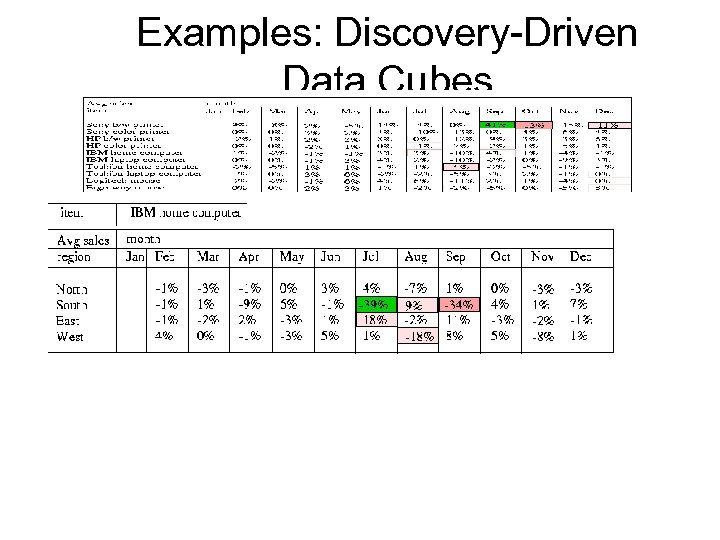Examples: Discovery-Driven Data Cubes

Data Warehouse Usage • Three kinds of data warehouse applications – Information processing • supports querying, basic statistical analysis, and reporting using crosstabs, tables, charts and graphs – Analytical processing • multidimensional analysis of data warehouse data • supports basic OLAP operations, slice-dice, drilling, pivoting – Data mining • knowledge discovery from hidden patterns • supports associations, constructing analytical models, performing classification and prediction, and presenting the mining results using visualization tools. • Differences among the three tasks

From On-Line Analytical Processing to On Line Analytical Mining (OLAM) • Why online analytical mining? – High quality of data in data warehouses • DW contains integrated, consistent, cleaned data – Available information processing structure surrounding data warehouses • ODBC, OLEDB, Web accessing, service facilities, reporting and OLAP tools – OLAP-based exploratory data analysis • mining with drilling, dicing, pivoting, etc. – On-line selection of data mining functions • integration and swapping of multiple mining functions, algorithms, and tasks. • Architecture of OLAM

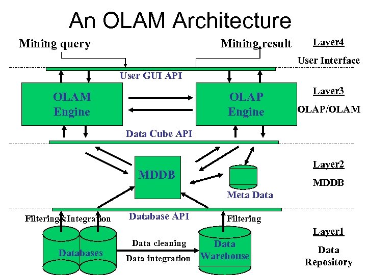An OLAM Architecture Mining query Mining result Layer 4 User Interface User GUI API OLAM Engine OLAP Engine Layer 3 OLAP/OLAM Data Cube API Layer 2 MDDB Meta Data Filtering&Integration Database API Filtering Layer 1 Databases Data cleaning Data integration Warehouse Data Repository