TOPIC Preferences — Important Concepts — u

TOPIC Preferences

- Important Concepts - u Fundamental Assumptions of Microeconomics What is microeconomics? – The study of how people fulfill unlimited wants with limited means. Fundamental Assumptions – Unlimited Desires/Nonsatiation – Limited Means/Scarcity u Cost/Benefit Approach to Decision Making – Rationality & Rational Self-Interest u Opportunity & Sunk Costs Positive & Normative Economic Analysis/Comparative Static Analysis u u Marginal Analysis – Marginal Benefits – Marginal Costs

Fundamentals of Cost/Benefit Decision Making Question: How does someone choose which wants to fulfill when they cannot fulfill them all? Economists Answer: By weighing the cost and benefit of fulfilling a want. If the benefit outweighs the cost, just do it! If the cost outweighs the benefit, don’t do it! Everything in microeconomics boils down to this simple cost benefit comparison!

Rationality u u Rational Decisions: – Decisions based on a cost/benefit comparison. Rationally Self-Interested Decisions: – Decisions based on a cost/benefit comparison where only the costs and benefits to an individual are considered, and not the costs and benefits to other individuals. Much of economic theory is developed around the assumption of rational self-interest, but there are economic theories that relax this assumption.

What makes something so simple, so hard? u Identifying what benefits are relevant to a decision can be difficult. u Identifying what costs are relevant to a decision can be difficult. u Adding up benefits and costs can be difficult.

Opportunity & Sunk Cost u Opportunity Cost: – The cost of engaging in one activity instead of another. – Understanding and weighing opportunity costs is paramount for good decision making. – But, opportunity costs are often neglected. u Sunk Cost: – Costs incurred regardless of whether or not you engage in an activity. – Understanding and ignoring sunk costs is paramount for good decision making. – But, opportunity cost are not always ignored.

Marginal Analysis u u Many decision we make in life are all or nothing propositions. – Should I buy a house or rent? – Should I go to college? – Should I get Married? – For these types of decisions, the basic cost/benefit comparison is a relatively straightforward yes or no answer. But, many decisions are not all or nothing propositions. – How many cans of soup should I buy? – How much money should I put in a savings account each month? – How many Prius will Toyota manufacture next year? – Marginal analysis extends our fundamental cost/benefit decision making framework to decisions where we must choose how much of an activity to engage in.

Marginal Costs & Benefits u u Marginal Cost: – The increase in the total cost that results from carrying out one additional unit of an activity Marginal Benefit: – The increase in the total benefit that results from carrying out one additional unit of an activity. Marginal Analysis says that we should increase our level of activity as long the marginal benefit exceeds the marginal cost!

Two Approaches to Modeling Individual Choice u Preference u Choice Based Approach

Preference Based Approach - Unobservable preference relation is primitive. - Specify a preference relation while imposing rationality axioms and then derive the implications of those axioms in terms of individual choice.

Choice Based Approach -- Observable choice behavior is primitive -- Specify consistency assumptions regarding observed choice and then derive the implications of these assumptions in terms of observed choices.

Preferences u To explain consumer behavior, economists assume that consumers have a set of tastes or preferences that they use to guide them in choosing between goods. These tastes differ substantially among individuals.

Preferences u Behavioral Postulate: A decisionmaker always chooses its most preferred alternative from its set of available alternatives. u So to model choice we must model decisionmakers’ preferences.

Preference Relations u Comparing two different consumption bundles, x and y: – strict preference: x is more preferred than is y. – weak preference: x is as at least as preferred as is y. – indifference: x is exactly as preferred as is y.

Preference Relations u Strict preference, weak preference and indifference are all preference relations. u Particularly, they are ordinal relations; i. e. they state only the order in which bundles are preferred.

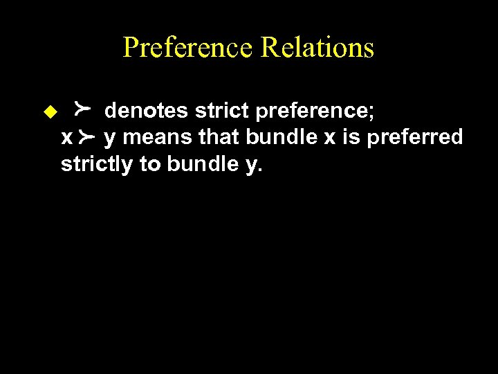Preference Relations p p u denotes strict preference; x y means that bundle x is preferred strictly to bundle y.

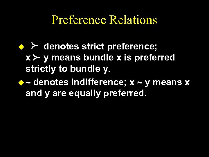Preference Relations p p denotes strict preference; x y means bundle x is preferred strictly to bundle y. u ~ denotes indifference; x ~ y means x and y are equally preferred. u

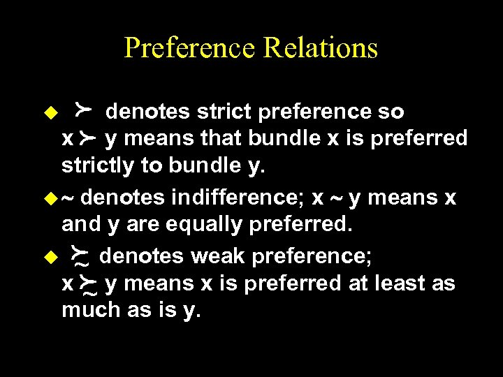Preference Relations p p denotes strict preference so x y means that bundle x is preferred strictly to bundle y. u ~ denotes indifference; x ~ y means x and y are equally preferred. u f denotes weak preference; ~ x f y means x is preferred at least as ~ as is y. much u

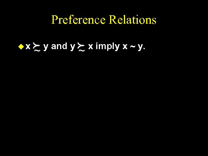Preference Relations ux f y and y f x imply x ~ y. ~ ~

Preference Relations f y and y f x imply x ~ y. ~ ~ u x f y and (not y f x) imply x ~ ~ ux y. p

Properties of Consumer Preferences u Economists make five critical assumptions about the properties of consumers’ preferences. For brevity, these properties are referred to as completeness, transitivity, more is better, continuity, and strict convexity.

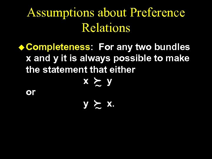Assumptions about Preference Relations u Completeness: For any two bundles x and y it is always possible to make the statement that either x f y ~ or y f x. ~

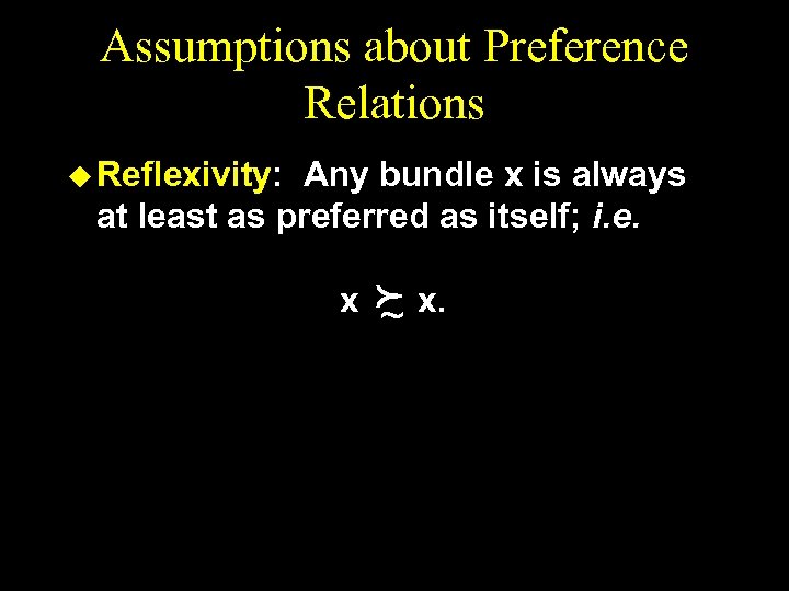Assumptions about Preference Relations u Reflexivity: Any bundle x is always at least as preferred as itself; i. e. x f x. ~

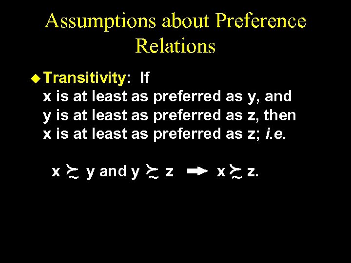Assumptions about Preference Relations u Transitivity: If x is at least as preferred as y, and y is at least as preferred as z, then x is at least as preferred as z; i. e. x f ~ y and y f ~ z x f z. ~

Indifference Curves u Take a reference bundle x’. The set of all bundles equally preferred to x’ is the indifference curve containing x’; the set of all bundles y ~ x’. u Since an indifference “curve” is not always a curve a better name might be an indifference “set”.

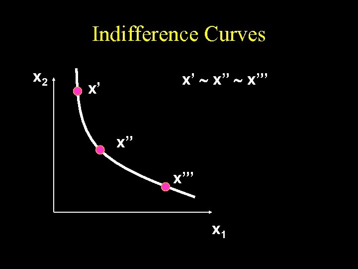Indifference Curves x 2 x’ ~ x”’ x’ x” x”’ x 1

Indifference Curves p x z y x 1 p x 2 y

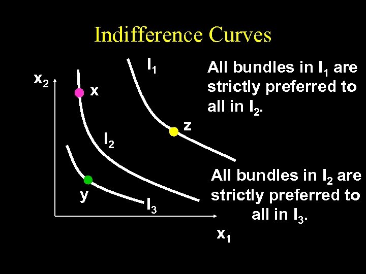Indifference Curves I 1 x 2 x z I 2 y I 3 All bundles in I 1 are strictly preferred to all in I 2. All bundles in I 2 are strictly preferred to all in I 3. x 1

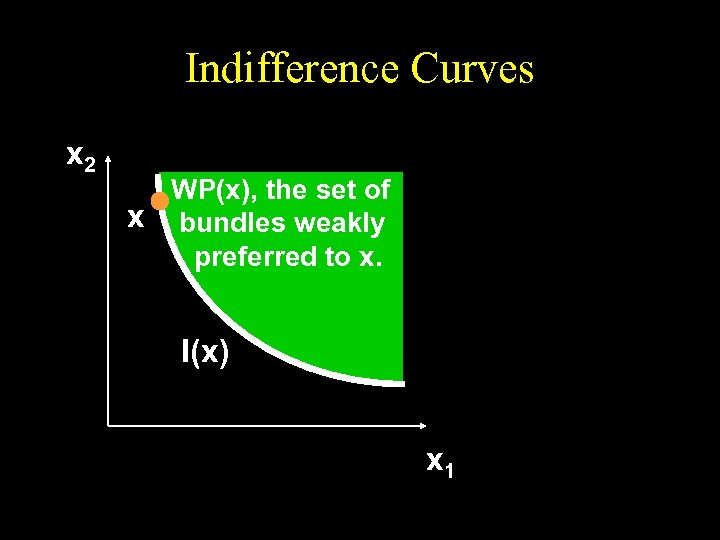Indifference Curves x 2 WP(x), the set of x bundles weakly preferred to x. I(x) I(x’) x 1

Indifference Curves x 2 WP(x), the set of x bundles weakly preferred to x. WP(x) includes I(x). x 1

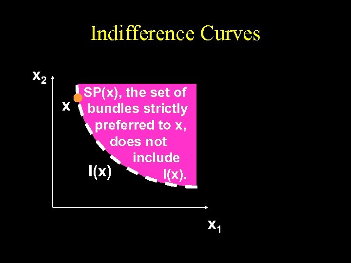Indifference Curves x 2 SP(x), the set of x bundles strictly preferred to x, does not include I(x). x 1

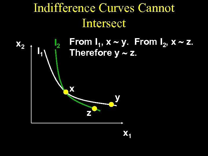Indifference Curves Cannot Intersect x 2 I 1 I 2 From I 1, x ~ y. From I 2, x ~ z. Therefore y ~ z. x y z x 1

Indifference Curves u All indifference curve maps must have four important properties: – Bundles on indifference curves farther from the origin are preferred to those on indifference curves closer to the origin. – There is an indifference curve through every possible bundle. – Indifference curve cannot cross. – Indifference curves slope downward.

Indifference Curves Cannot Intersect I 1 I 2 From I 1, x ~ y. From I 2, x ~ z. Therefore y ~ z. But from I 1 and I 2 we see y z, a contradiction. x y p x 2 z x 1

Slopes of Indifference Curves u When more of a commodity is always preferred, the commodity is a good. u If every commodity is a good then indifference curves are negatively sloped.

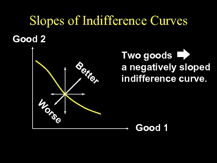Slopes of Indifference Curves Good 2 Be tte r W or se Two goods a negatively sloped indifference curve. Good 1

Slopes of Indifference Curves u If less of a commodity is always preferred then the commodity is a bad.

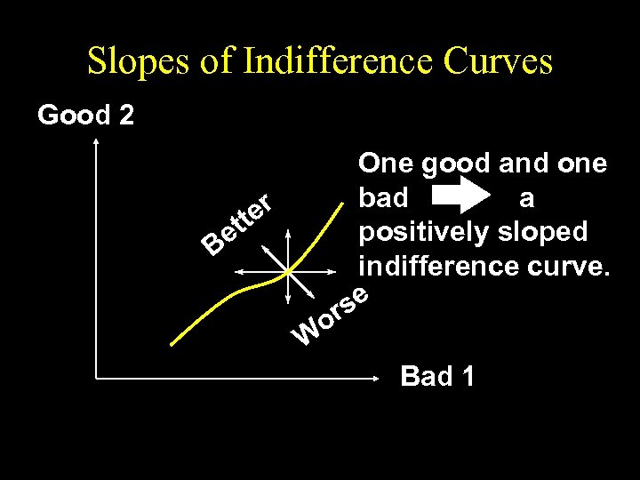Slopes of Indifference Curves Good 2 One good and one bad a r tte positively sloped e B indifference curve. se or W Bad 1

Extreme Cases of Indifference Curves; Perfect Substitutes u If a consumer always regards units of commodities 1 and 2 as equivalent, then the commodities are perfect substitutes and only the total amount of the two commodities in bundles determines their preference rank-order.

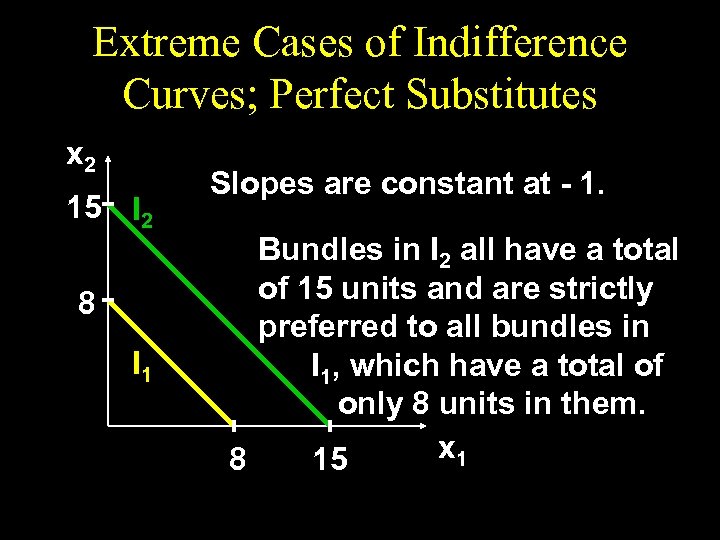Extreme Cases of Indifference Curves; Perfect Substitutes x 2 15 I 2 8 I 1 Slopes are constant at - 1. Bundles in I 2 all have a total of 15 units and are strictly preferred to all bundles in I 1, which have a total of only 8 units in them. x 1 8 15

Extreme Cases of Indifference Curves; Perfect Complements u If a consumer always consumes commodities 1 and 2 in fixed proportion (e. g. one-to-one), then the commodities are perfect complements and only the number of pairs of units of the two commodities determines the preference rank-order of bundles.

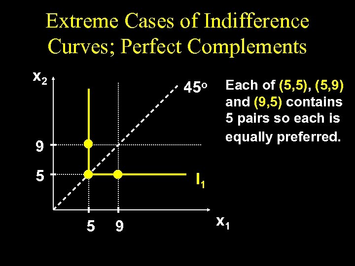Extreme Cases of Indifference Curves; Perfect Complements x 2 45 o 9 5 Each of (5, 5), (5, 9) and (9, 5) contains 5 pairs so each is equally preferred. I 1 5 9 x 1

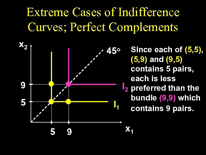Extreme Cases of Indifference Curves; Perfect Complements x 2 Since each of (5, 5), (5, 9) and (9, 5) contains 5 pairs, each is less I 2 preferred than the bundle (9, 9) which I 1 contains 9 pairs. 45 o 9 5 5 9 x 1

Preferences Exhibiting Satiation u. A bundle strictly preferred to any other is a satiation point or a bliss point. u What do indifference curves look like for preferences exhibiting satiation?

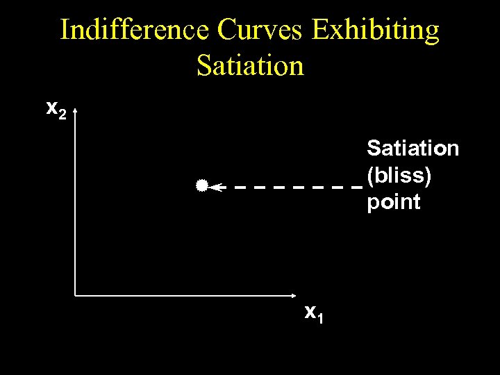Indifference Curves Exhibiting Satiation x 2 Satiation (bliss) point x 1

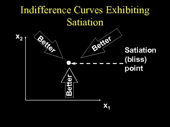Indifference Curves Exhibiting Satiation Be tte r ter et B Better x 2 x 1 Satiation (bliss) point

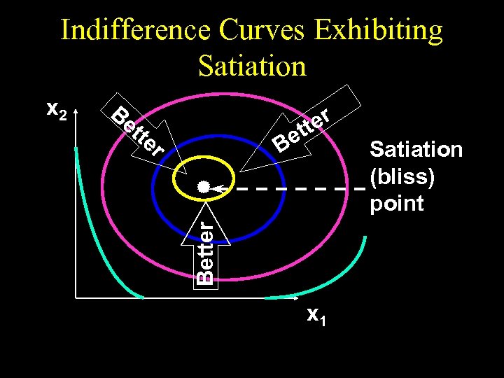Indifference Curves Exhibiting Satiation Be tte r ter et B Better x 2 x 1 Satiation (bliss) point

Indifference Curves for Discrete Commodities u. A commodity is infinitely divisible if it can be acquired in any quantity; e. g. water or cheese. u A commodity is discrete if it comes in unit lumps of 1, 2, 3, … and so on; e. g. aircraft, ships and refrigerators.

Indifference Curves for Discrete Commodities u Suppose commodity 2 is an infinitely divisible good (gasoline) while commodity 1 is a discrete good (aircraft). What do indifference “curves” look like?

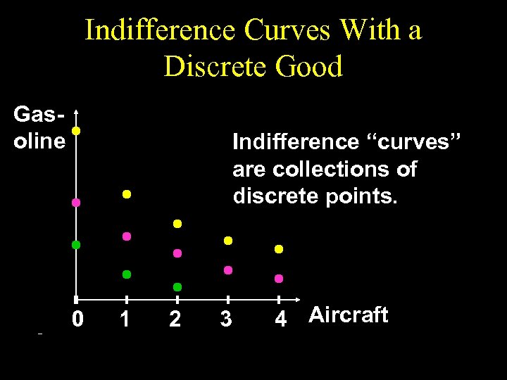Indifference Curves With a Discrete Good Gasoline Indifference “curves” are collections of discrete points. 0 1 2 3 4 Aircraft

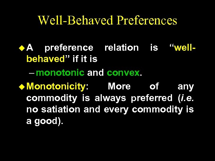Well-Behaved Preferences u. A preference relation is “wellbehaved” if it is – monotonic and convex. u Monotonicity: More of any commodity is always preferred (i. e. no satiation and every commodity is a good).

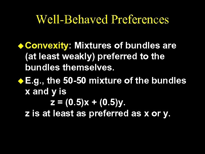Well-Behaved Preferences u Convexity: Mixtures of bundles are (at least weakly) preferred to the bundles themselves. u E. g. , the 50 -50 mixture of the bundles x and y is z = (0. 5)x + (0. 5)y. z is at least as preferred as x or y.

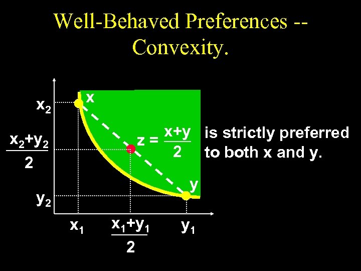Well-Behaved Preferences -Convexity. x x 2 x+y is strictly preferred z= 2 to both x and y. x 2+y 2 2 y y 2 x 1+y 1 2 y 1

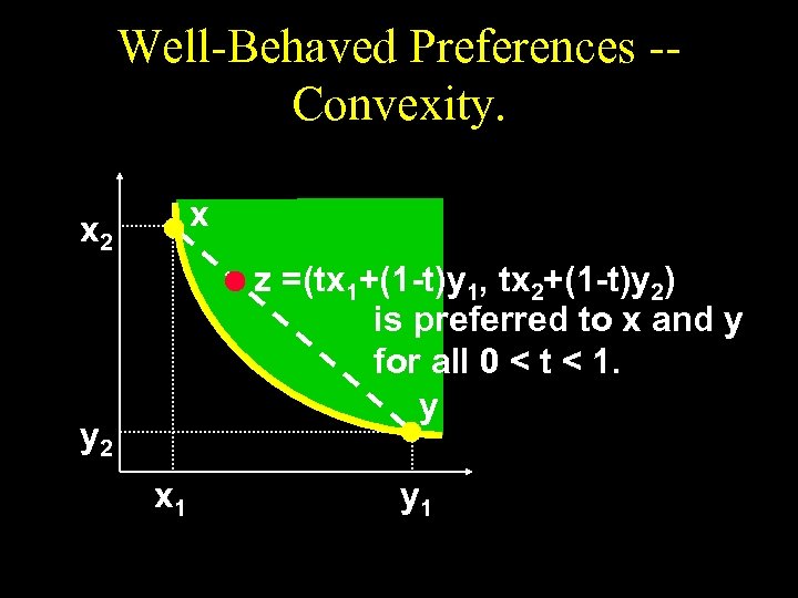Well-Behaved Preferences -Convexity. x x 2 z =(tx 1+(1 -t)y 1, tx 2+(1 -t)y 2) is preferred to x and y for all 0 < t < 1. y y 2 x 1 y 1

Well-Behaved Preferences -Convexity. x x 2 y 2 x 1 Preferences are strictly convex when all mixtures z are strictly z preferred to their component bundles x and y. y y 1

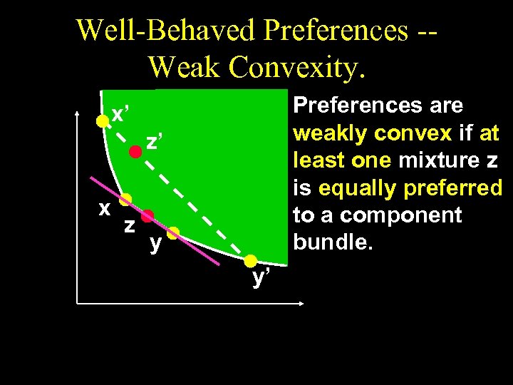Well-Behaved Preferences -Weak Convexity. Preferences are weakly convex if at least one mixture z is equally preferred to a component bundle. x’ z’ x z y y’

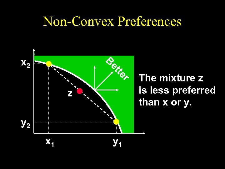Non-Convex Preferences B x 2 r te et z y 2 x 1 y 1 The mixture z is less preferred than x or y.

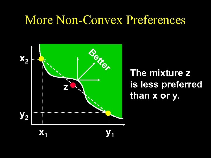More Non-Convex Preferences B r te et x 2 z y 2 x 1 y 1 The mixture z is less preferred than x or y.

Slopes of Indifference Curves u The slope of an indifference curve is its marginal rate-of-substitution (MRS). u How can a MRS be calculated?

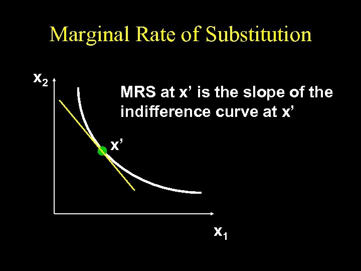Marginal Rate of Substitution x 2 MRS at x’ is the slope of the indifference curve at x’ x’ x 1

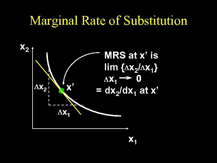Marginal Rate of Substitution x 2 D x 2 x’ MRS at x’ is lim {Dx 2/Dx 1} D x 1 0 = dx 2/dx 1 at x’ D x 1

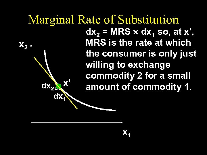Marginal Rate of Substitution x 2 dx 2 x’ dx 1 dx 2 = MRS ´ dx 1 so, at x’, MRS is the rate at which the consumer is only just willing to exchange commodity 2 for a small amount of commodity 1. x 1

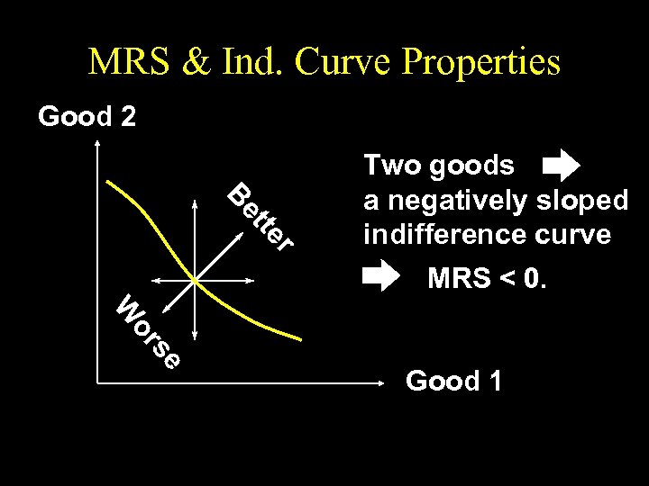MRS & Ind. Curve Properties Good 2 r er tte ett Be B Two goods a negatively sloped indifference curve MRS < 0. se se or or W W Good 1

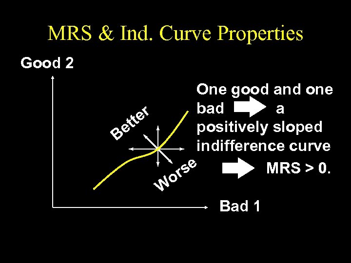MRS & Ind. Curve Properties Good 2 One good and one bad a r tte positively sloped e B indifference curve MRS > 0. se r o W Bad 1

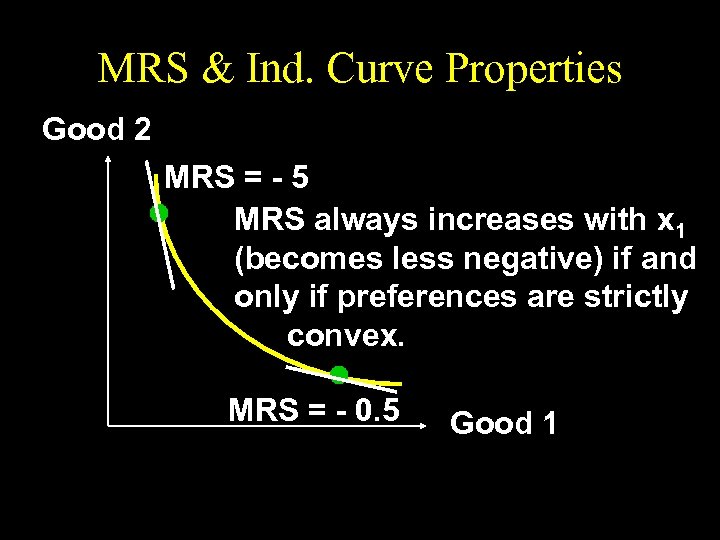MRS & Ind. Curve Properties Good 2 MRS = - 5 MRS always increases with x 1 (becomes less negative) if and only if preferences are strictly convex. MRS = - 0. 5 Good 1

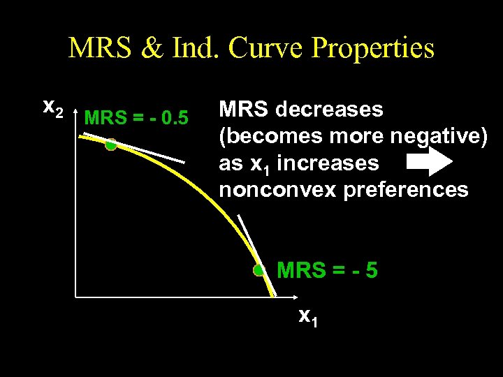MRS & Ind. Curve Properties x 2 MRS = - 0. 5 MRS decreases (becomes more negative) as x 1 increases nonconvex preferences MRS = - 5 x 1

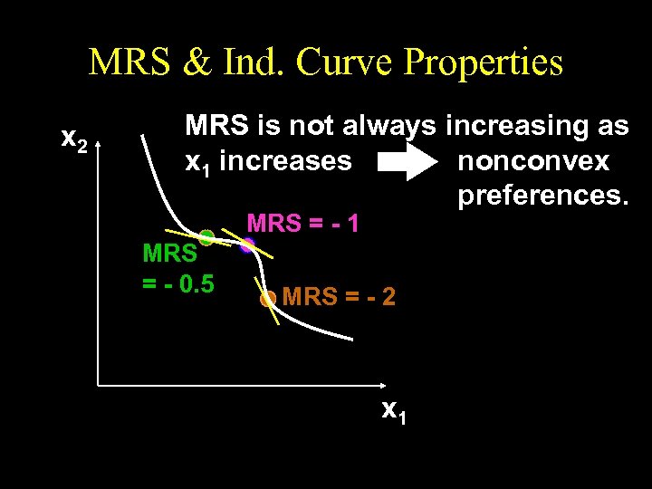MRS & Ind. Curve Properties x 2 MRS is not always increasing as x 1 increases nonconvex preferences. MRS = - 1 MRS = - 0. 5 MRS = - 2 x 1