748b8cec0b761708265380336ef88b79.ppt
- Количество слайдов: 107
 Topic 4: Regional Economics
 Part A: Data on Housing Cycles
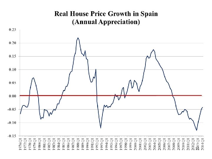
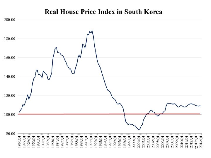
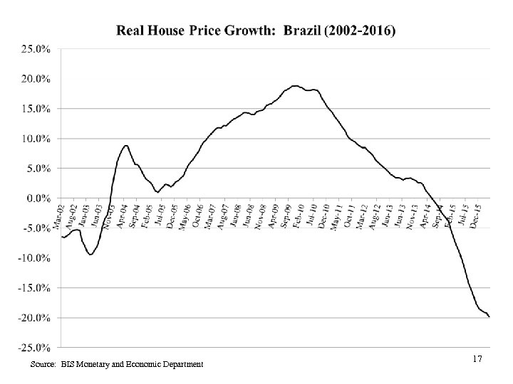
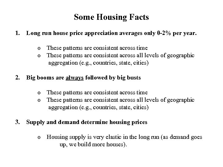 Some Housing Facts 1. Long run house price appreciation averages only 0 -2% per year. o o 2. Big booms are always followed by big busts o o 3. These patterns are consistent across time These patterns are consistent across all levels of geographic aggregation (e. g. , countries, state, cities) Supply and demand determine housing prices o Housing supply is very elastic in the long run (as demand goes up, we build more houses).
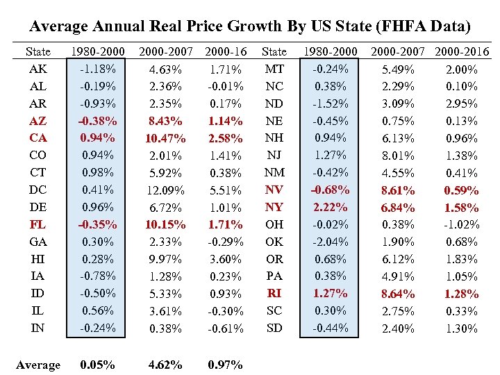 Average Annual Real Price Growth By US State (FHFA Data) State AK AL AR AZ CA CO CT DC DE FL GA HI IA ID IL IN 1980 -2000 -1. 18% -0. 19% -0. 93% -0. 38% 0. 94% 0. 98% 0. 41% 0. 96% -0. 35% 0. 30% 0. 28% -0. 78% -0. 50% 0. 56% -0. 24% 2000 -2007 2000 -16 4. 63% 1. 71% 2. 36% -0. 01% 2. 35% 0. 17% 8. 43% 1. 14% 10. 47% 2. 58% 2. 01% 1. 41% 5. 92% 0. 38% 12. 09% 5. 51% 6. 72% 1. 01% 10. 15% 1. 71% 2. 33% -0. 29% 9. 97% 3. 60% 1. 28% 0. 23% 5. 33% 0. 93% 3. 61% -0. 30% 0. 38% -0. 61% State MT NC ND NE NH NJ NM NV NY OH OK OR PA RI SC SD 1980 -2000 -0. 24% 0. 38% -1. 52% -0. 45% 0. 94% 1. 27% -0. 42% -0. 68% 2. 22% -0. 02% -2. 04% 0. 68% 0. 38% 1. 27% 0. 30% -0. 44% 2000 -2007 2000 -2016 5. 49% 2. 00% 2. 29% 0. 10% 3. 09% 2. 95% 0. 75% 0. 13% 6. 13% 0. 96% 8. 01% 1. 38% 4. 55% 0. 41% 8. 61% 0. 59% 6. 84% 1. 58% 0. 38% -1. 02% 1. 90% 0. 68% 6. 12% 1. 83% 4. 91% 1. 05% 8. 64% 1. 28% 2. 75% 0. 33% 2. 40% 1. 30% 4 Average 0. 05% 4. 62% 0. 97%
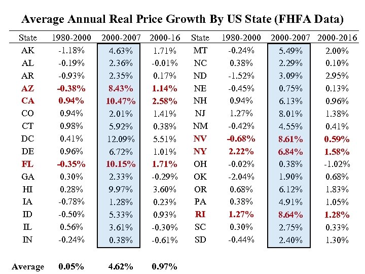 Average Annual Real Price Growth By US State (FHFA Data) State AK AL AR AZ CA CO CT DC DE FL GA HI IA ID IL IN 1980 -2000 -1. 18% -0. 19% -0. 93% -0. 38% 0. 94% 0. 98% 0. 41% 0. 96% -0. 35% 0. 30% 0. 28% -0. 78% -0. 50% 0. 56% -0. 24% 2000 -2007 2000 -16 4. 63% 1. 71% 2. 36% -0. 01% 2. 35% 0. 17% 8. 43% 1. 14% 10. 47% 2. 58% 2. 01% 1. 41% 5. 92% 0. 38% 12. 09% 5. 51% 6. 72% 1. 01% 10. 15% 1. 71% 2. 33% -0. 29% 9. 97% 3. 60% 1. 28% 0. 23% 5. 33% 0. 93% 3. 61% -0. 30% 0. 38% -0. 61% State MT NC ND NE NH NJ NM NV NY OH OK OR PA RI SC SD 1980 -2000 -0. 24% 0. 38% -1. 52% -0. 45% 0. 94% 1. 27% -0. 42% -0. 68% 2. 22% -0. 02% -2. 04% 0. 68% 0. 38% 1. 27% 0. 30% -0. 44% 2000 -2007 2000 -2016 5. 49% 2. 00% 2. 29% 0. 10% 3. 09% 2. 95% 0. 75% 0. 13% 6. 13% 0. 96% 8. 01% 1. 38% 4. 55% 0. 41% 8. 61% 0. 59% 6. 84% 1. 58% 0. 38% -1. 02% 1. 90% 0. 68% 6. 12% 1. 83% 4. 91% 1. 05% 8. 64% 1. 28% 2. 75% 0. 33% 2. 40% 1. 30% 5 Average 0. 05% 4. 62% 0. 97%
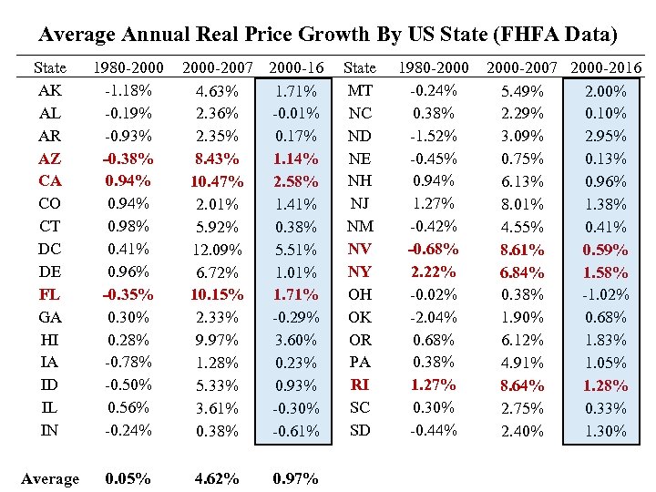 Average Annual Real Price Growth By US State (FHFA Data) State AK AL AR AZ CA CO CT DC DE FL GA HI IA ID IL IN 1980 -2000 -1. 18% -0. 19% -0. 93% -0. 38% 0. 94% 0. 98% 0. 41% 0. 96% -0. 35% 0. 30% 0. 28% -0. 78% -0. 50% 0. 56% -0. 24% 2000 -2007 2000 -16 4. 63% 1. 71% 2. 36% -0. 01% 2. 35% 0. 17% 8. 43% 1. 14% 10. 47% 2. 58% 2. 01% 1. 41% 5. 92% 0. 38% 12. 09% 5. 51% 6. 72% 1. 01% 10. 15% 1. 71% 2. 33% -0. 29% 9. 97% 3. 60% 1. 28% 0. 23% 5. 33% 0. 93% 3. 61% -0. 30% 0. 38% -0. 61% State MT NC ND NE NH NJ NM NV NY OH OK OR PA RI SC SD 1980 -2000 -0. 24% 0. 38% -1. 52% -0. 45% 0. 94% 1. 27% -0. 42% -0. 68% 2. 22% -0. 02% -2. 04% 0. 68% 0. 38% 1. 27% 0. 30% -0. 44% 2000 -2007 2000 -2016 5. 49% 2. 00% 2. 29% 0. 10% 3. 09% 2. 95% 0. 75% 0. 13% 6. 13% 0. 96% 8. 01% 1. 38% 4. 55% 0. 41% 8. 61% 0. 59% 6. 84% 1. 58% 0. 38% -1. 02% 1. 90% 0. 68% 6. 12% 1. 83% 4. 91% 1. 05% 8. 64% 1. 28% 2. 75% 0. 33% 2. 40% 1. 30% 6 Average 0. 05% 4. 62% 0. 97%
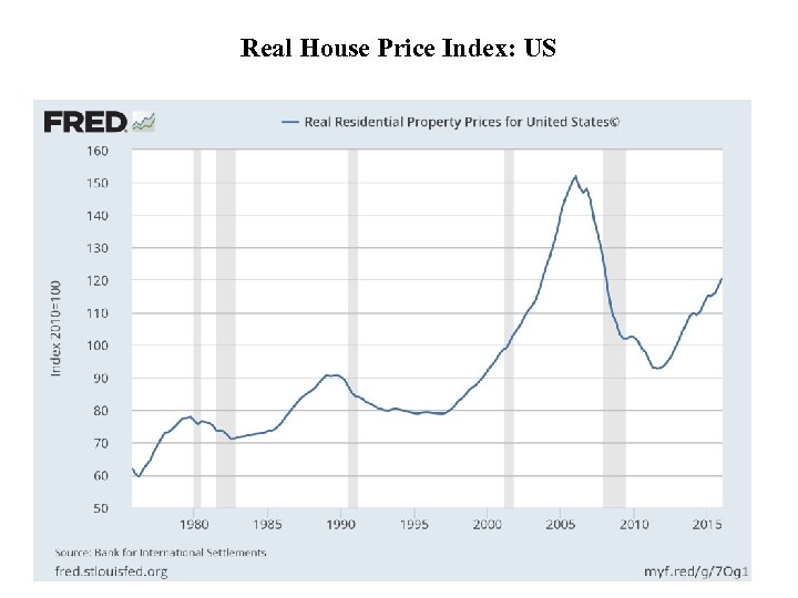 Real House Price Index: US 7
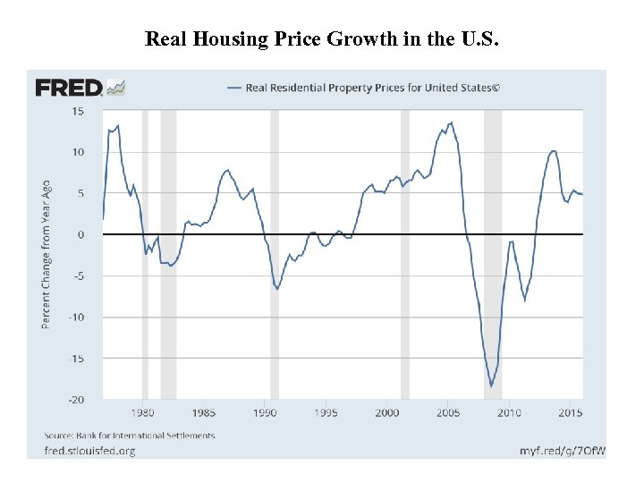 Real Housing Price Growth in the U. S. 8
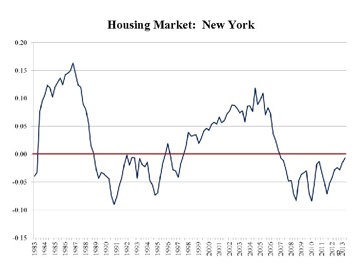 Housing Market: New York 9
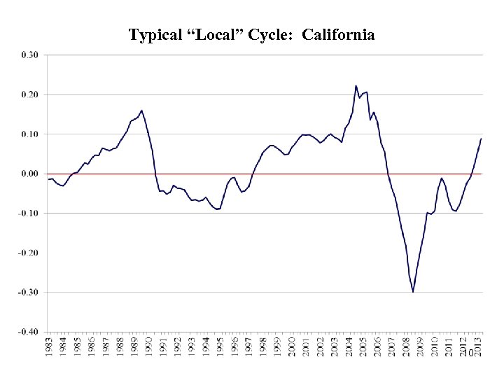 Typical “Local” Cycle: California 10
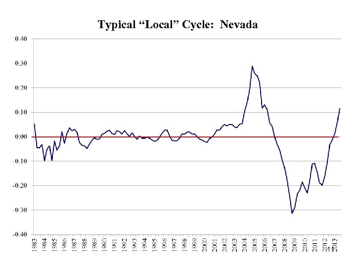 Typical “Local” Cycle: Nevada 11
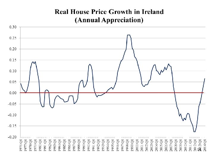
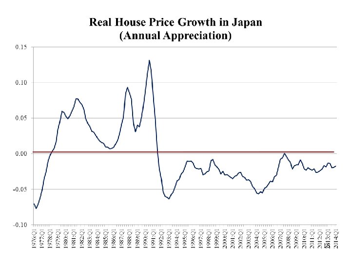
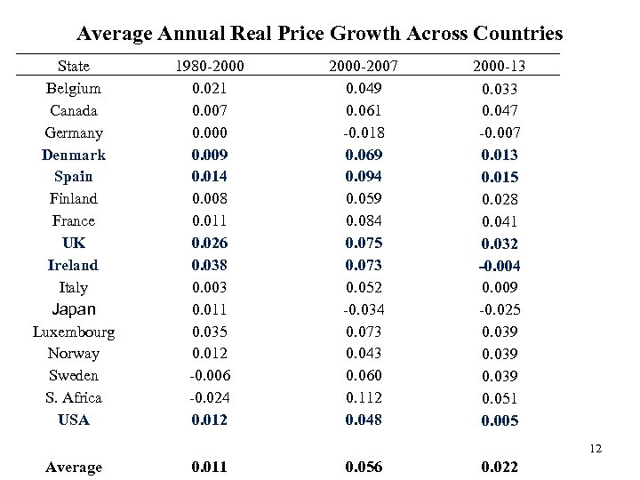 Average Annual Real Price Growth Across Countries State Belgium Canada Germany Denmark Spain Finland France UK Ireland Italy Japan Luxembourg Norway Sweden S. Africa USA 1980 -2000 0. 021 0. 007 0. 000 0. 009 0. 014 0. 008 0. 011 0. 026 0. 038 0. 003 0. 011 0. 035 0. 012 -0. 006 -0. 024 0. 012 2000 -2007 0. 049 0. 061 -0. 018 0. 069 0. 094 0. 059 0. 084 0. 075 0. 073 0. 052 -0. 034 0. 073 0. 043 0. 060 0. 112 0. 048 2000 -13 0. 033 0. 047 -0. 007 0. 013 0. 015 0. 028 0. 041 0. 032 -0. 004 0. 009 -0. 025 0. 039 0. 051 0. 005 12 Average 0. 011 0. 056 0. 022
 13
13
 14
14
 15
15
 16
16
 Source: BIS Monetary and Economic Department 17
 Part B: Some Models of Spatial Equilibrium
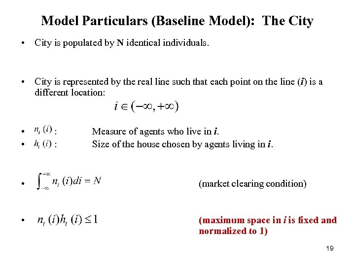 Model Particulars (Baseline Model): The City • City is populated by N identical individuals. • City is represented by the real line such that each point on the line (i) is a different location: • • : : Measure of agents who live in i. Size of the house chosen by agents living in i. • (market clearing condition) • (maximum space in i is fixed and normalized to 1) 19
 Household Preferences Static model:
 Construction
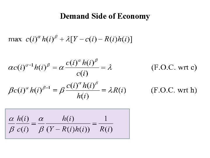 Demand Side of Economy
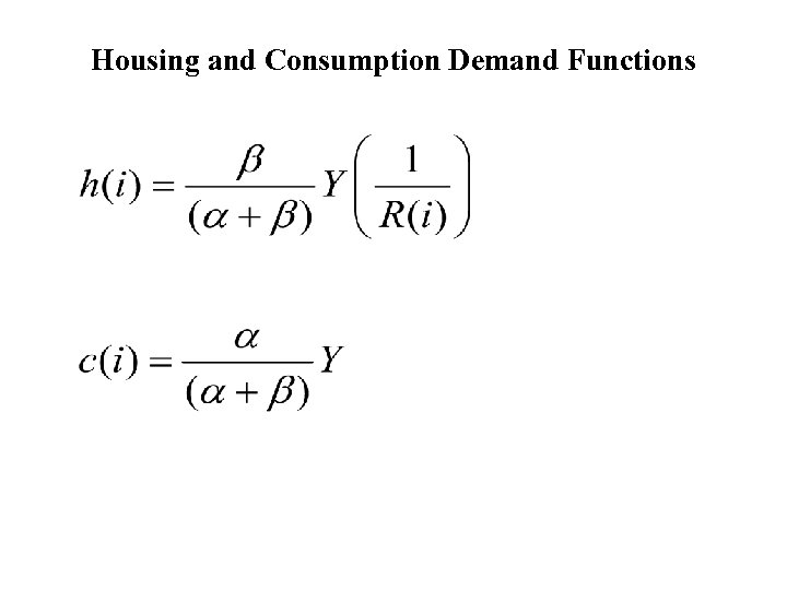 Housing and Consumption Demand Functions
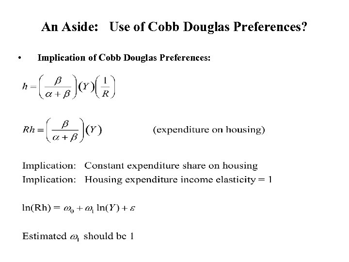 An Aside: Use of Cobb Douglas Preferences? • Implication of Cobb Douglas Preferences:
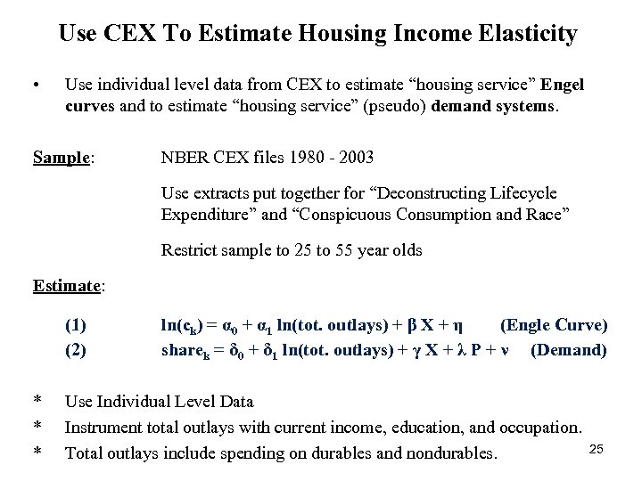 Use CEX To Estimate Housing Income Elasticity • Use individual level data from CEX to estimate “housing service” Engel curves and to estimate “housing service” (pseudo) demand systems. Sample: NBER CEX files 1980 - 2003 Use extracts put together for “Deconstructing Lifecycle Expenditure” and “Conspicuous Consumption and Race” Restrict sample to 25 to 55 year olds Estimate: (1) (2) * * * ln(ck) = α 0 + α 1 ln(tot. outlays) + β X + η (Engle Curve) sharek = δ 0 + δ 1 ln(tot. outlays) + γ X + λ P + ν (Demand) Use Individual Level Data Instrument total outlays with current income, education, and occupation. Total outlays include spending on durables and nondurables. 25
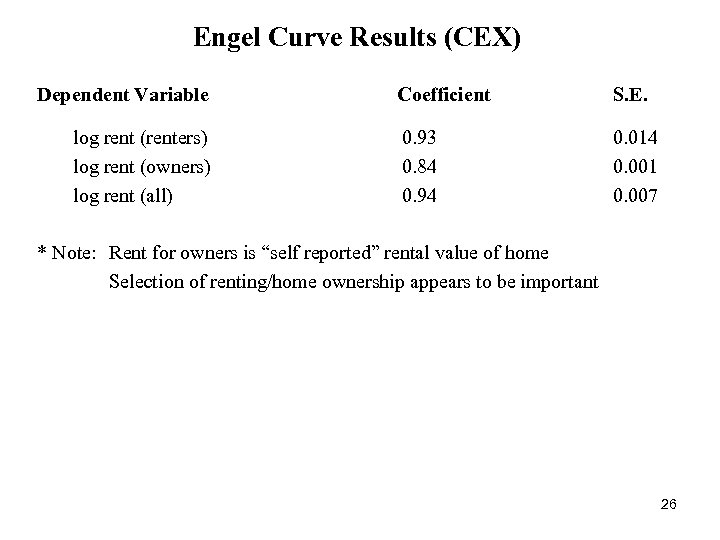 Engel Curve Results (CEX) Dependent Variable log rent (renters) log rent (owners) log rent (all) Coefficient S. E. 0. 93 0. 84 0. 94 0. 014 0. 001 0. 007 * Note: Rent for owners is “self reported” rental value of home Selection of renting/home ownership appears to be important 26
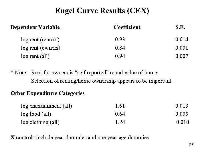 Engel Curve Results (CEX) Dependent Variable log rent (renters) log rent (owners) log rent (all) Coefficient S. E. 0. 93 0. 84 0. 94 0. 014 0. 001 0. 007 * Note: Rent for owners is “self reported” rental value of home Selection of renting/home ownership appears to be important Other Expenditure Categories log entertainment (all) log food (all) log clothing (all) 1. 61 0. 64 1. 24 0. 013 0. 005 0. 010 X controls include year dummies and one year age dummies 27
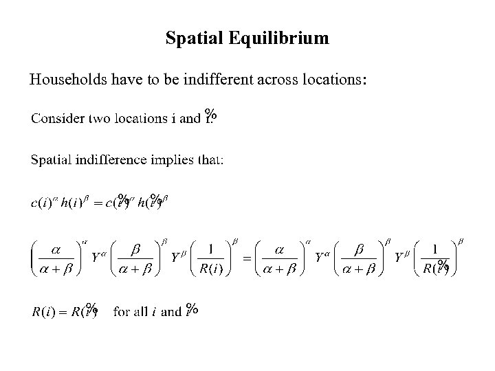 Spatial Equilibrium Households have to be indifferent across locations:
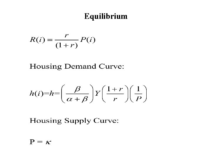 Equilibrium
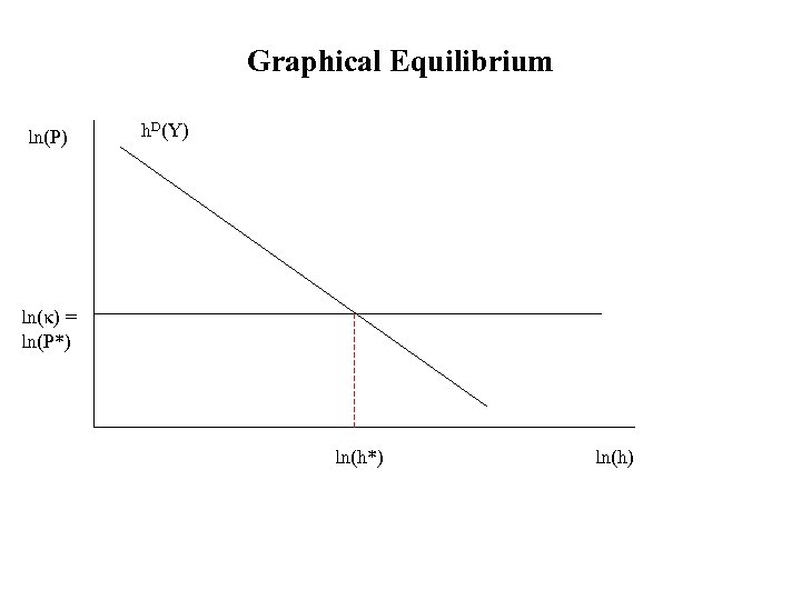 Graphical Equilibrium ln(P) h. D(Y) ln(κ) = ln(P*) ln(h)
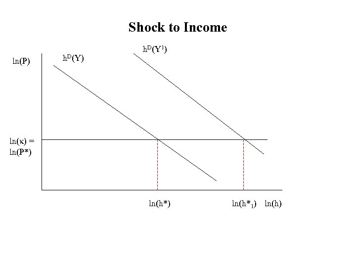 Shock to Income ln(P) h. D(Y 1) ln(κ) = ln(P*) ln(h*1) ln(h)
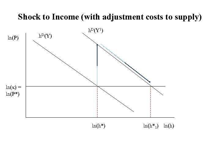 Shock to Income (with adjustment costs to supply) ln(P) h. D(Y 1) ln(κ) = ln(P*) ln(h*1) ln(h)
 Some Conclusions (Base Model) • If supply is perfectly elastic in the long run (land is available and construction costs are fixed), then: Prices will be fixed in the long run Demand shocks will have no effect on prices in the long run. Short run amplification of prices could be do to adjustment costs. Model has “static” optimization. Similar results with dynamic optimization (and expectations – with some caveats) • Notice – location – per se – is not important in this analysis. All locations are the same.
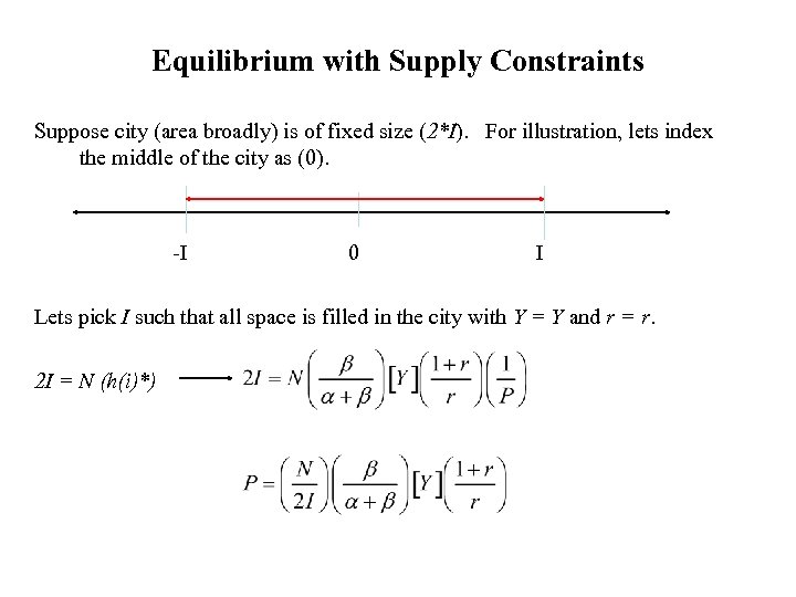 Equilibrium with Supply Constraints Suppose city (area broadly) is of fixed size (2*I). For illustration, lets index the middle of the city as (0). -I 0 I Lets pick I such that all space is filled in the city with Y = Y and r = r. 2 I = N (h(i)*)
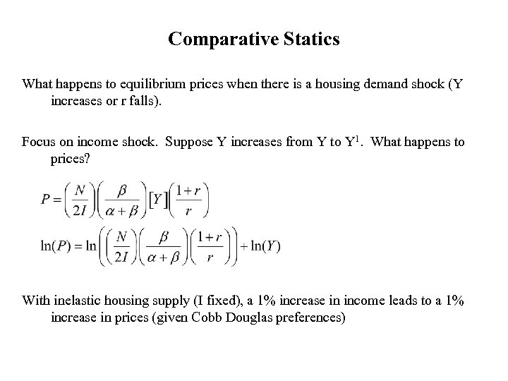 Comparative Statics What happens to equilibrium prices when there is a housing demand shock (Y increases or r falls). Focus on income shock. Suppose Y increases from Y to Y 1. What happens to prices? With inelastic housing supply (I fixed), a 1% increase in income leads to a 1% increase in prices (given Cobb Douglas preferences)
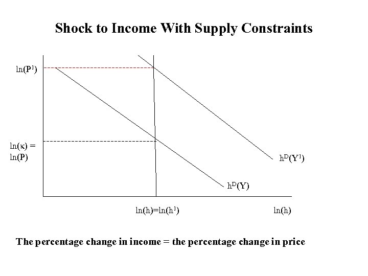 Shock to Income With Supply Constraints ln(P 1) ln(κ) = ln(P) h. D(Y 1) h. D(Y) ln(h)=ln(h 1) ln(h) The percentage change in income = the percentage change in price
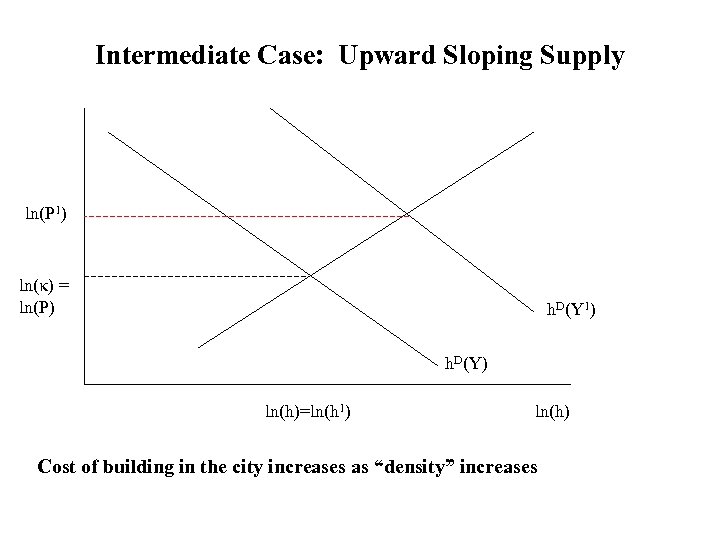 Intermediate Case: Upward Sloping Supply ln(P 1) ln(κ) = ln(P) h. D(Y 1) h. D(Y) ln(h)=ln(h 1) ln(h) Cost of building in the city increases as “density” increases
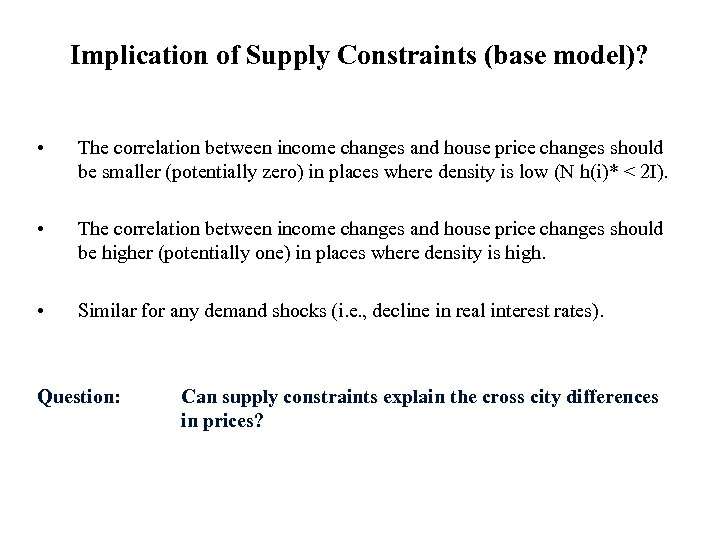 Implication of Supply Constraints (base model)? • The correlation between income changes and house price changes should be smaller (potentially zero) in places where density is low (N h(i)* < 2 I). • The correlation between income changes and house price changes should be higher (potentially one) in places where density is high. • Similar for any demand shocks (i. e. , decline in real interest rates). Question: Can supply constraints explain the cross city differences in prices?
 Topel and Rosen (1988) “Housing Investment in the United States” (JPE) • First paper to formally approach housing price dynamics. • Uses aggregate data • Finds that housing supply is relatively elastic in the long run Long run elasticity is much higher than short run elasticity. Long run was about “one year” • Implication: Long run annual aggregate home price appreciation for the U. S. is small.
 Siaz (2010) “On Local Housing Supply Elasticity (QJE 2010) • Estimates housing supply elasticities by city. • Uses a measure of “developable” land in the city. • What makes land “undevelopable”? Gradient Coverage of water • Differences across cities changes the potential supply responsiveness across cities to a demand shock (some places are more supply elastic in the short run).
 Can Supply Constraints Explain Cycles? “Housing Dynamics” by Glaeser et al. Calibrated spatial equilibrium model Match data on construction (building permits) and housing prices using time series and cross MSA variation. Find that supply constraints cannot explain housing price cycles. Their explanation: Negatively serially correlated demand shocks.
 What Could Be Missing From Simple Model? • Add in reasons for agglomeration. • Long literature looking at housing prices across areas with agglomeration. • Most of these focus on “production” agglomerations. • We will lay out one of the simplest models – Muth (1969), Alonzo (1964), Mills (1967) • Locations are no longer identical. There is a center business district in the area where people work (indexed as point (0) for our analysis). • Households who live (i) distance from center business district must pay additional transportation cost of τi.
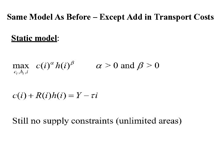 Same Model As Before – Except Add in Transport Costs Static model:
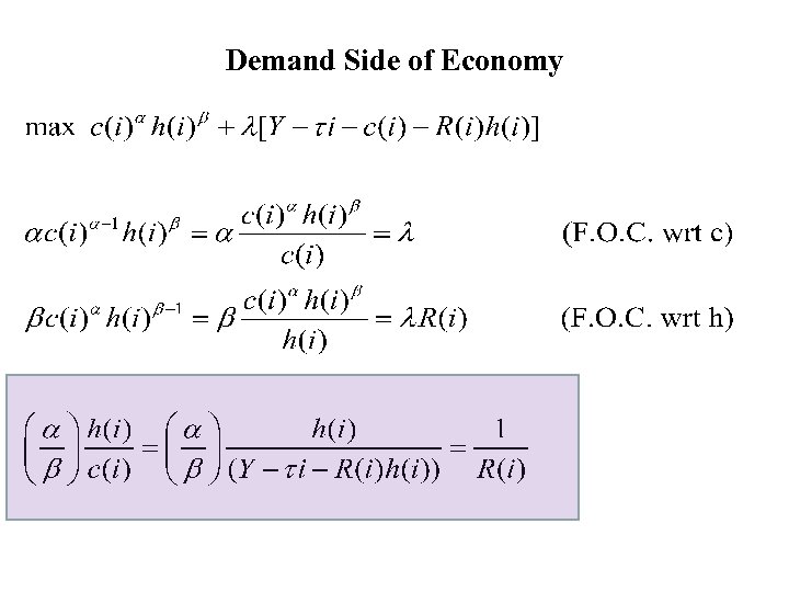 Demand Side of Economy
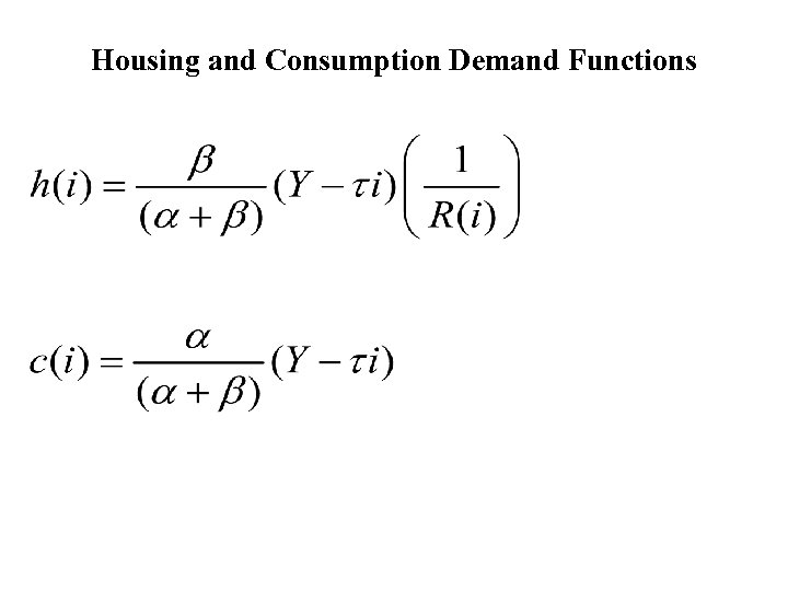 Housing and Consumption Demand Functions
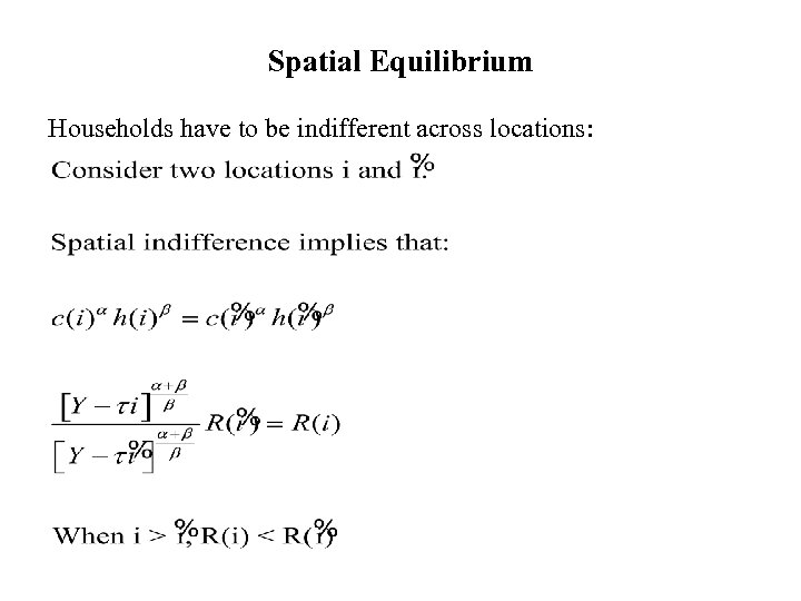 Spatial Equilibrium Households have to be indifferent across locations:
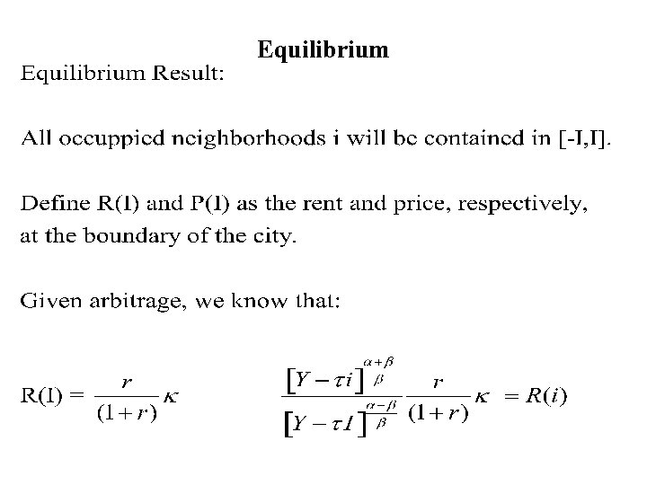 Equilibrium
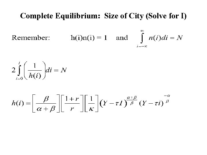 Complete Equilibrium: Size of City (Solve for I)
 Some Algebra (if my algebra is correct…)
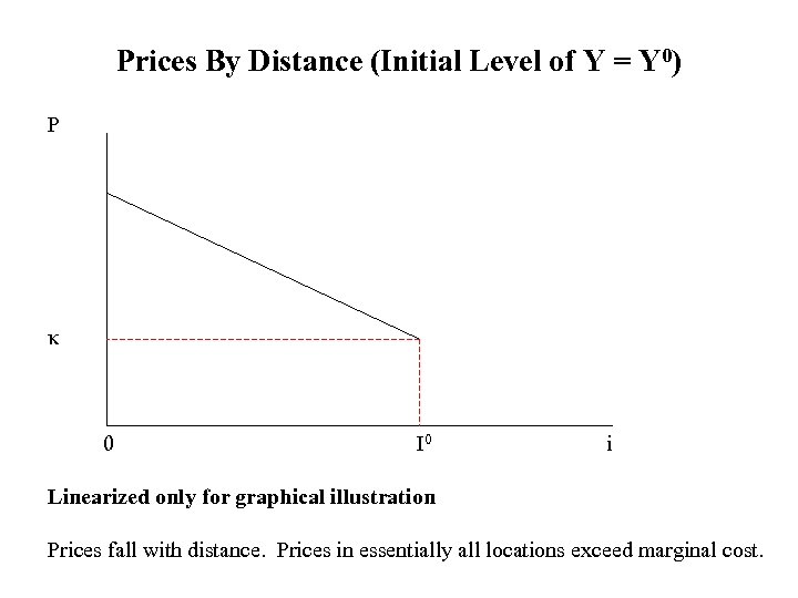 Prices By Distance (Initial Level of Y = Y 0) P κ 0 I 0 i Linearized only for graphical illustration Prices fall with distance. Prices in essentially all locations exceed marginal cost.
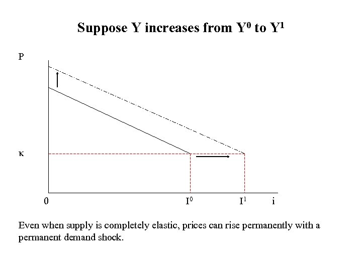 Suppose Y increases from Y 0 to Y 1 P κ 0 I 1 i Even when supply is completely elastic, prices can rise permanently with a permanent demand shock.
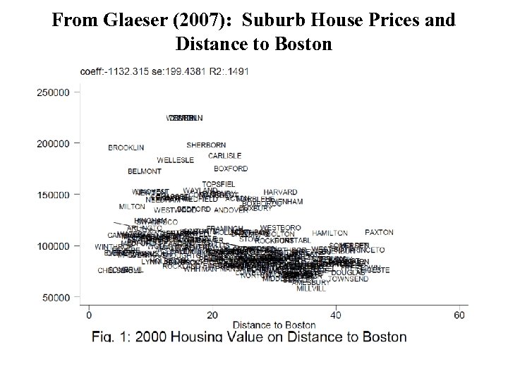 From Glaeser (2007): Suburb House Prices and Distance to Boston
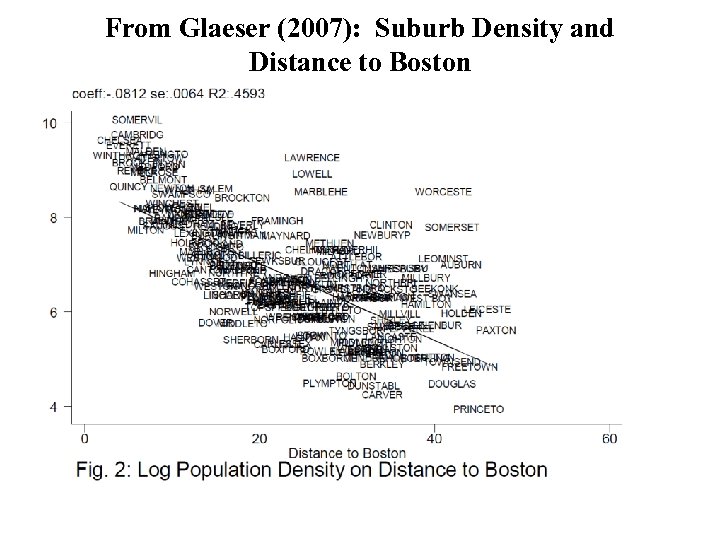 From Glaeser (2007): Suburb Density and Distance to Boston
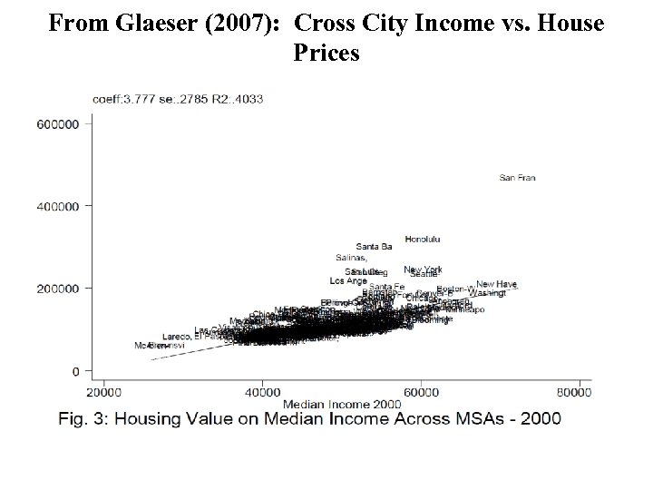 From Glaeser (2007): Cross City Income vs. House Prices
 A Quick Review of Spatial Equilibrium Models • Cross city differences? Long run price differences across cities with no differential supply constraints. Strength of the center business district (size of τ) drives some of differences in long run price appreciations across city. • Is it big enough? • Fall in τ will lead to bigger cities (suburbs) and lower prices in center city (i = 0).
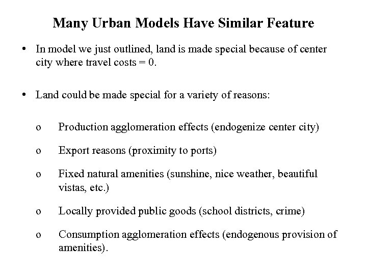 Many Urban Models Have Similar Feature • In model we just outlined, land is made special because of center city where travel costs = 0. • Land could be made special for a variety of reasons: o Production agglomeration effects (endogenize center city) o Export reasons (proximity to ports) o Fixed natural amenities (sunshine, nice weather, beautiful vistas, etc. ) o Locally provided public goods (school districts, crime) o Consumption agglomeration effects (endogenous provision of amenities).
 Part C: “Endogenous Gentrification and House Price Dynamics” (Guerrieri, Hartley, and Hurst)
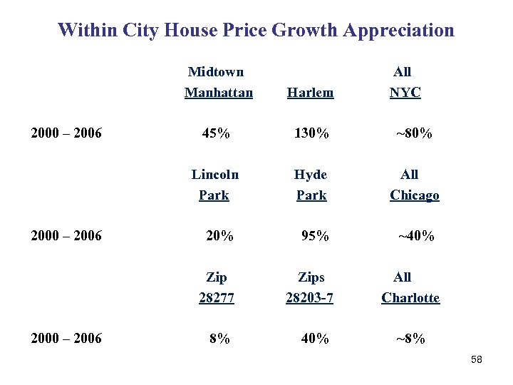 Within City House Price Growth Appreciation Midtown Manhattan 2000 – 2006 45% 130% ~80% Hyde Park All Chicago 20% 95% Zip 28277 2000 – 2006 Harlem Lincoln Park 2000 – 2006 All NYC Zips 28203 -7 8% 40% ~40% All Charlotte ~8% 58
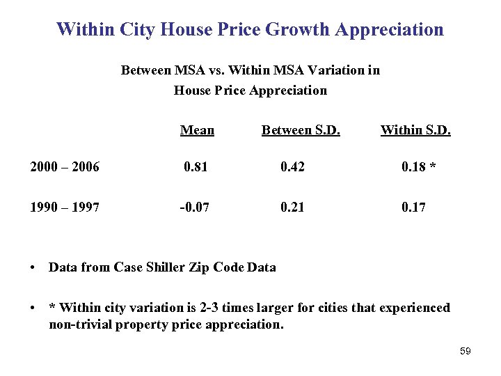 Within City House Price Growth Appreciation Between MSA vs. Within MSA Variation in House Price Appreciation Mean Between S. D. Within S. D. 2000 – 2006 0. 81 0. 42 0. 18 * 1990 – 1997 -0. 07 0. 21 0. 17 • Data from Case Shiller Zip Code Data • * Within city variation is 2 -3 times larger for cities that experienced non-trivial property price appreciation. 59
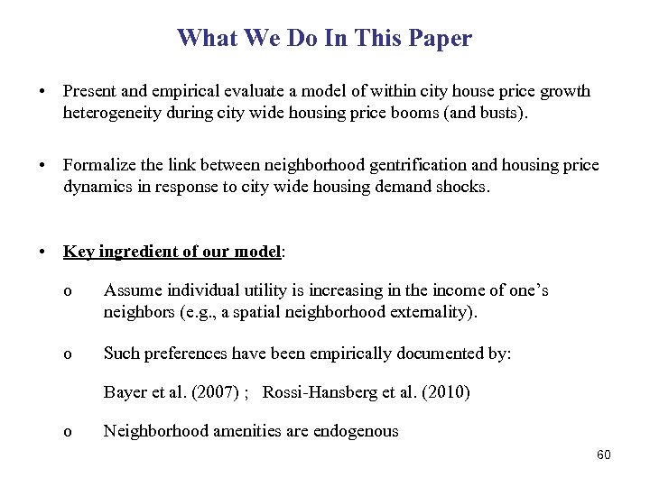 What We Do In This Paper • Present and empirical evaluate a model of within city house price growth heterogeneity during city wide housing price booms (and busts). • Formalize the link between neighborhood gentrification and housing price dynamics in response to city wide housing demand shocks. • Key ingredient of our model: o Assume individual utility is increasing in the income of one’s neighbors (e. g. , a spatial neighborhood externality). o Such preferences have been empirically documented by: Bayer et al. (2007) ; Rossi-Hansberg et al. (2010) o Neighborhood amenities are endogenous 60
 Where Do the Preferences Come From • Our preference structure is a catch all for many potential stories. • As a result, we do not take a stand on what – in particular – people like about “rich” neighborhoods. - Lower crime (dislike poor neighborhoods) - Quality and extent of public goods (like schools) – could be through expenditures or peer effects. - Increasing returns to scale in the provision of local service amenities (restaurants, entertainment options, etc. ). 61
 Mechanism for Within City Price Movements • With the externality, any land occupied by rich people will be of higher value than land occupied by non-rich people. – Can explain the within city differences in prices such that rich neighborhoods have higher land prices (Becker and Murphy (2003)). • Anything that increases the demand for housing of rich people (i. e. , an influx of new rich people) increases the value of the land onto which they move. o New/expanding rich will migrate to the poor neighborhoods that directly border the existing rich neighborhoods (to maximize value of the externality) o The poor will get priced out of these border neighborhoods. o We refer to this process as “endogenous” gentrification. 62
 Document Empirical Support for the Model • Use variation from Bartik-type shocks across cities (cities that get an exogenous labor demand shock based on initial industry mix). • For cities that get larger Bartik shocks: 1. House prices in the city as a whole appreciate more. 2. Poor neighborhoods that directly abut rich neighborhoods appreciate the most (both relative to rich neighborhoods and poor neighborhoods that are far from rich neighborhoods). 3. Poor neighborhoods that directly abut rich neighborhoods show much more signs of gentrification (income growth of residents) relative to other poor neighborhoods. 4. These patterns occur in the 1980 s, 1990 s, and 2000 s. 63
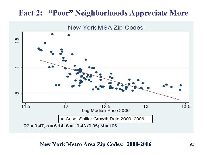 Fact 2: “Poor” Neighborhoods Appreciate More New York Metro Area Zip Codes: 2000 -2006 64
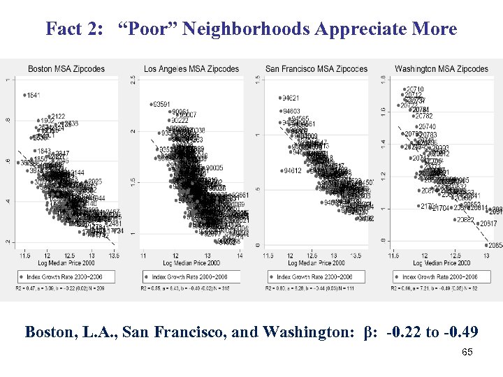 Fact 2: “Poor” Neighborhoods Appreciate More Boston, L. A. , San Francisco, and Washington: β: -0. 22 to -0. 49 65
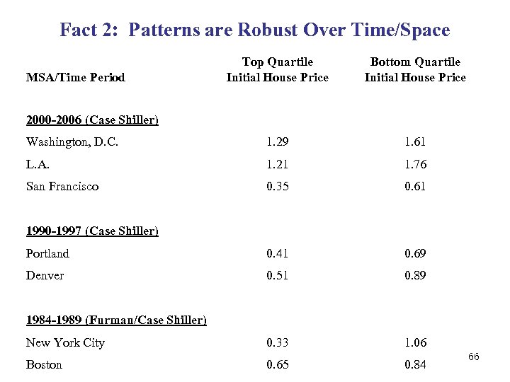 Fact 2: Patterns are Robust Over Time/Space Top Quartile Initial House Price Bottom Quartile Initial House Price Washington, D. C. 1. 29 1. 61 L. A. 1. 21 1. 76 San Francisco 0. 35 0. 61 Portland 0. 41 0. 69 Denver 0. 51 0. 89 New York City 0. 33 1. 06 Boston 0. 65 0. 84 MSA/Time Period 2000 -2006 (Case Shiller) 1990 -1997 (Case Shiller) 1984 -1989 (Furman/Case Shiller) 66
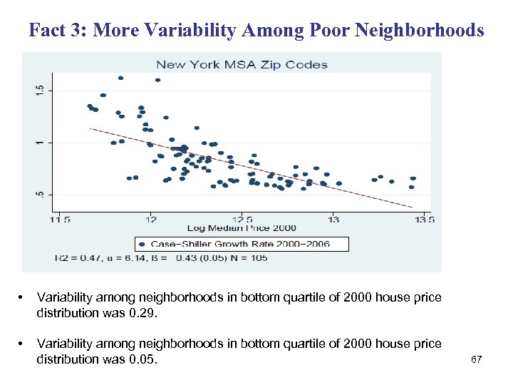 Fact 3: More Variability Among Poor Neighborhoods • Variability among neighborhoods in bottom quartile of 2000 house price distribution was 0. 29. • Variability among neighborhoods in bottom quartile of 2000 house price distribution was 0. 05. 67
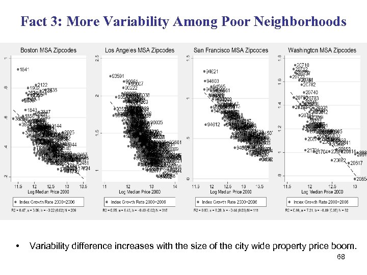 Fact 3: More Variability Among Poor Neighborhoods • Variability difference increases with the size of the city wide property price boom. 68
 Summary of Facts • Tremendous amount of within city house price variation. • Variation across zip codes/census tracts within a city is of similar magnitude as the well studied cross city variation. • Poor neighborhoods within a city appreciate most during city wide housing booms. The more the city as a whole appreciates, the bigger the differential between rich and poor neighborhoods within a city. • There is much greater variation in house price appreciation rates among poor neighborhoods. The variation increases with the size of the city wide housing boom. • All the facts are interesting and should be explored more fully in subsequent theoretical and empirical work. • Our subsequent theory and empirical work only focuses on trying to explain the variation among the poor neighborhoods. 69
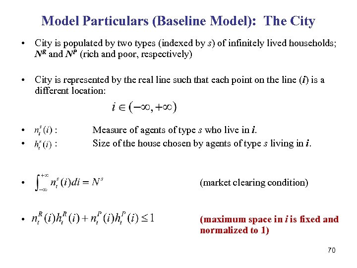 Model Particulars (Baseline Model): The City • City is populated by two types (indexed by s) of infinitely lived households; NR and NP (rich and poor, respectively) • City is represented by the real line such that each point on the line (i) is a different location: • • : : Measure of agents of type s who live in i. Size of the house chosen by agents of type s living in i. • (market clearing condition) • (maximum space in i is fixed and normalized to 1) 70
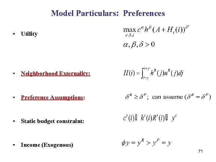 Model Particulars: Preferences • Utility • Neighborhood Externality: • Preference Assumptions: • Static budget constraint: • Income (Exogenous) 71
 Comments on the Model 1. No distinction between poor people and farm land (nothing interesting about the poor except they are not rich). - Could include a negative externality from living near the poor. We have not done that at this time. 2. No bounds on the city (or mechanisms to bound the city – like transport costs or location specific amenities). 3. Only two types of income (rich and poor). 4. Only one dimension of preference externality. 5. Neighborhoods are of fixed size (do not allow building up). 6. Externality is over space occupied by rich people (not amount of rich people). 7. No uncertainty (more on this later if time allows). 72
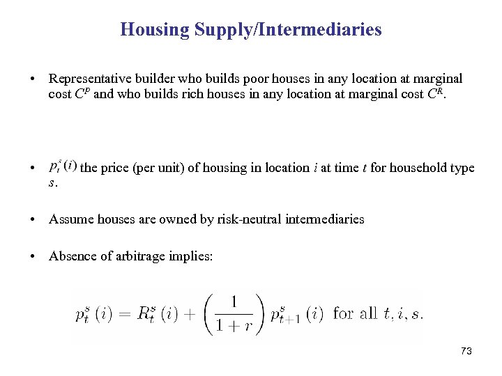 Housing Supply/Intermediaries • Representative builder who builds poor houses in any location at marginal cost CP and who builds rich houses in any location at marginal cost CR. • s. the price (per unit) of housing in location i at time t for household type • Assume houses are owned by risk-neutral intermediaries • Absence of arbitrage implies: 73
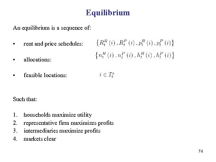 Equilibrium An equilibrium is a sequence of: • rent and price schedules: • allocations: • feasible locations: Such that: 1. 2. 3. 4. households maximize utility representative firm maximizes profits intermediaries maximize profits markets clear 74
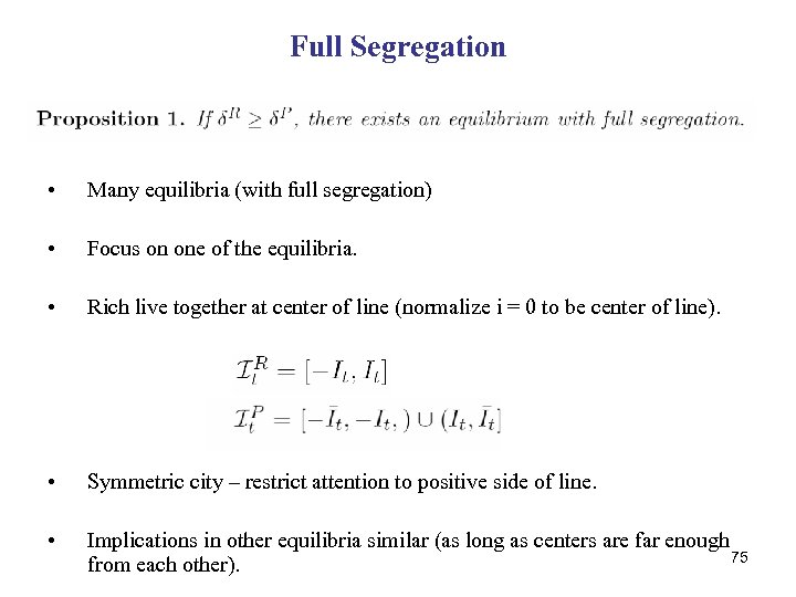 Full Segregation • Many equilibria (with full segregation) • Focus on one of the equilibria. • Rich live together at center of line (normalize i = 0 to be center of line). • Symmetric city – restrict attention to positive side of line. • Implications in other equilibria similar (as long as centers are far enough 75 from each other).
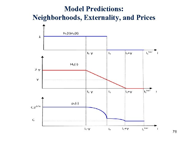 Model Predictions: Neighborhoods, Externality, and Prices 76
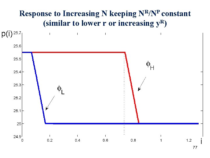 Response to Increasing N keeping NR/NP constant (similar to lower r or increasing y. R) 77
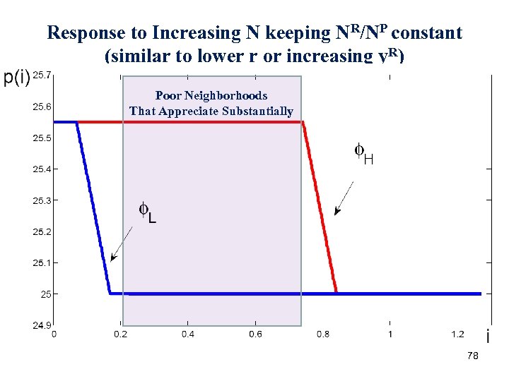 Response to Increasing N keeping NR/NP constant (similar to lower r or increasing y. R) Poor Neighborhoods That Appreciate Substantially 78
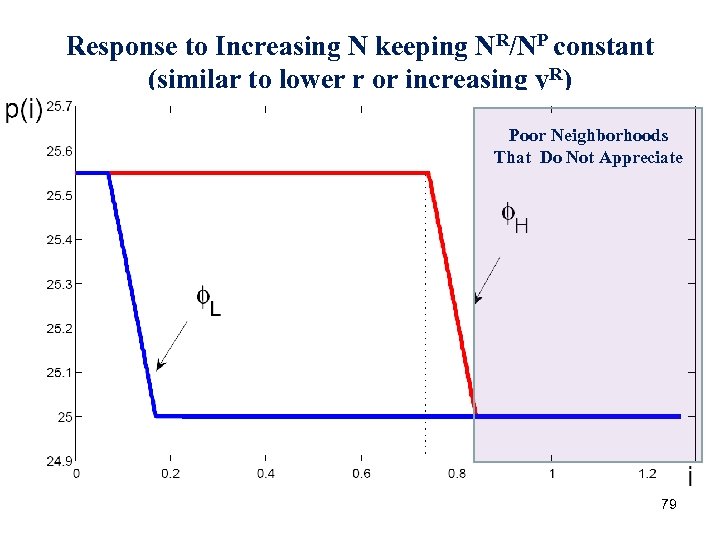 Response to Increasing N keeping NR/NP constant (similar to lower r or increasing y. R) Poor Neighborhoods That Do Not Appreciate 79
 Implications of Model: Within City • Lower priced neighborhoods are more price responsive than high priced neighborhoods to positive demand shocks. • It is the low priced neighborhoods in close proximity to the high priced neighborhoods that appreciate the most when there is a positive housing demand shock. • The low priced neighborhoods in close proximity to the high priced neighborhoods that appreciate the most do so because they gentrify (rich people move into those neighborhoods). 80
 Implications of Model: Cross City • Mechanism is relevant in that it can also explain differences in price appreciation across cities. • Higher income growth (NR increase) within a city leads to higher house price appreciation (P) at the city level, all else equal. - Define P as the weighted average of prices within the city. The city P just reflects the aggregation of the neighborhood p’s. • The stronger the externality (δ), the larger the price growth at the city level (P), all else equal. 81
 Rest of Paper • Test predictions of model using: o Within city price movements o Exogenous “Bartik” shocks to city as a whole (i. e. , manufacturing declines, finance booms, etc. ). o Show strong support for the model Poor neighborhoods on the border of rich neighborhoods are more likely to appreciate in response to a city wide labor demand shock (relative to other equally poor neighborhoods). These neighborhoods also experience a rapid turnover in population type (i. e. , they got richer). 82
 Part D: Local Labor Market Adjustment (Blanchard and Katz)
 How Do Locations Respond to Local Shocks? • Continue our theme about thinking about regional economics (house prices are one part of that). • The direct mechanism: • What implications do mobility have on the response of labor supply, wages, and unemployment to local economic shocks? • Some work: Mobility. Blanchard/Katz “Regional Evolutions” (Brookings, 1992) Topel “Local Labor Markets” (JPE, 1986)
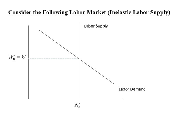 Consider the Following Labor Market (Inelastic Labor Supply) Labor Supply Labor Demand
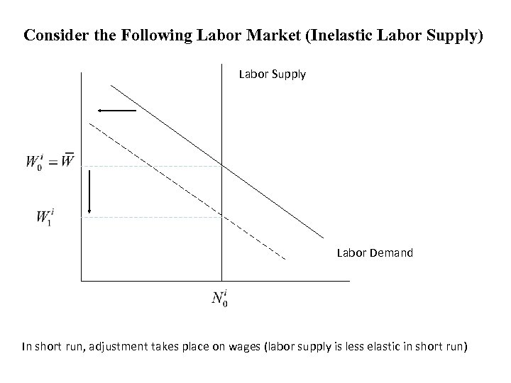 Consider the Following Labor Market (Inelastic Labor Supply) Labor Supply Labor Demand In short run, adjustment takes place on wages (labor supply is less elastic in short run)
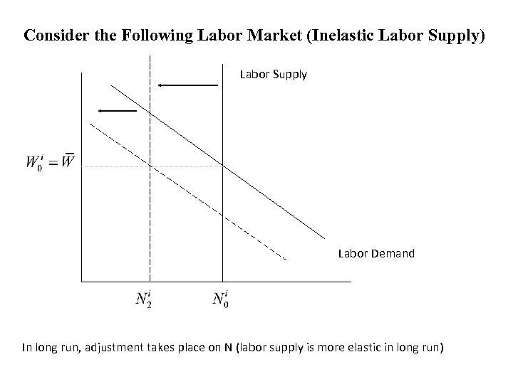 Consider the Following Labor Market (Inelastic Labor Supply) Labor Supply Labor Demand In long run, adjustment takes place on N (labor supply is more elastic in long run)
 What is the Mechanism? • In/out migration of workers…. .
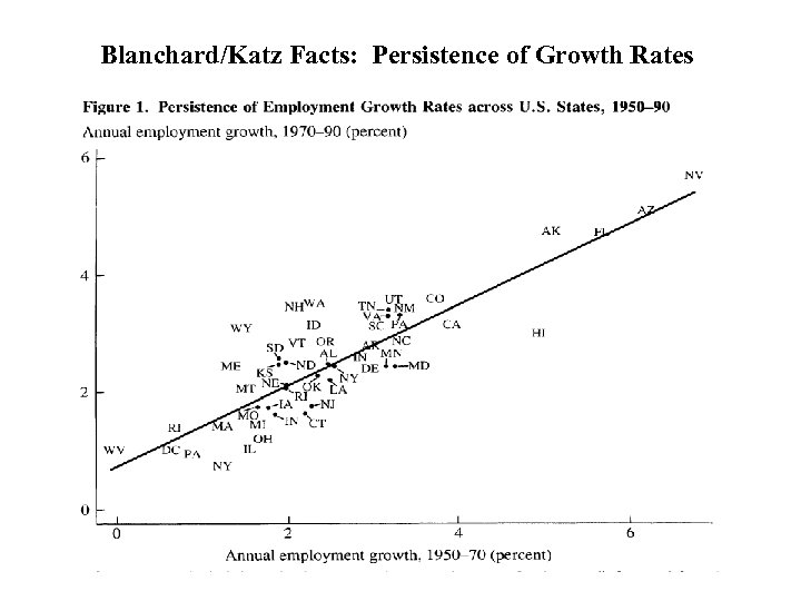 Blanchard/Katz Facts: Persistence of Growth Rates
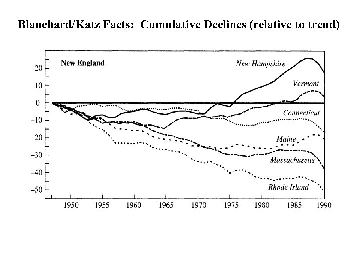 Blanchard/Katz Facts: Cumulative Declines (relative to trend)
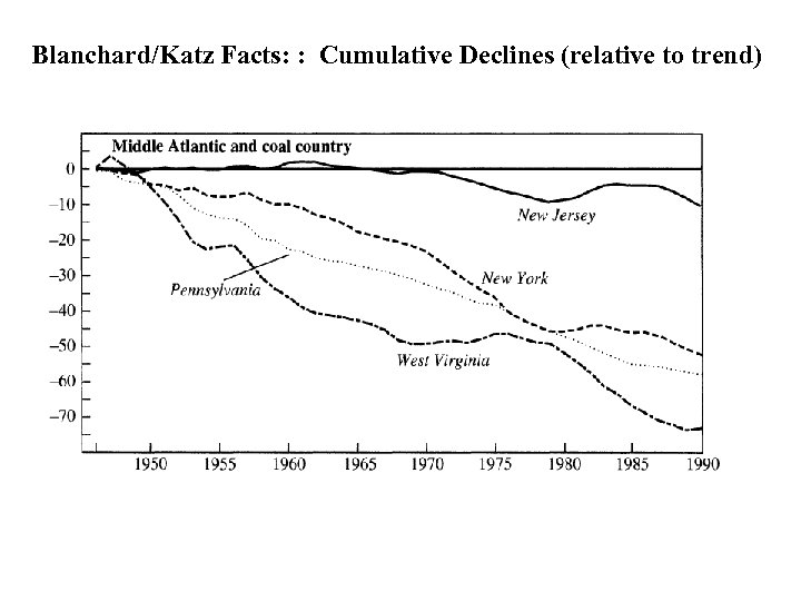 Blanchard/Katz Facts: : Cumulative Declines (relative to trend)
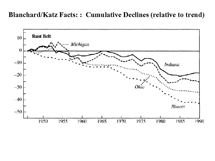 Blanchard/Katz Facts: : Cumulative Declines (relative to trend)
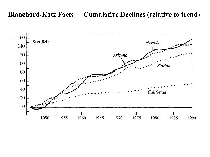 Blanchard/Katz Facts: : Cumulative Declines (relative to trend)
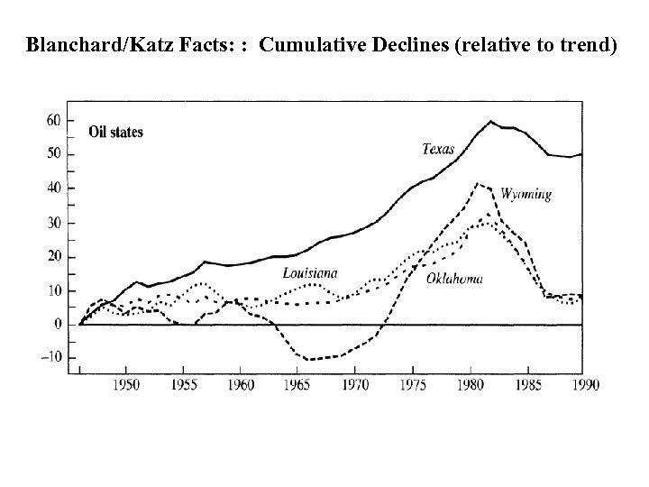 Blanchard/Katz Facts: : Cumulative Declines (relative to trend)
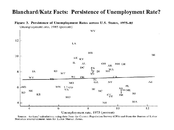 Blanchard/Katz Facts: Persistence of Unemployment Rate?
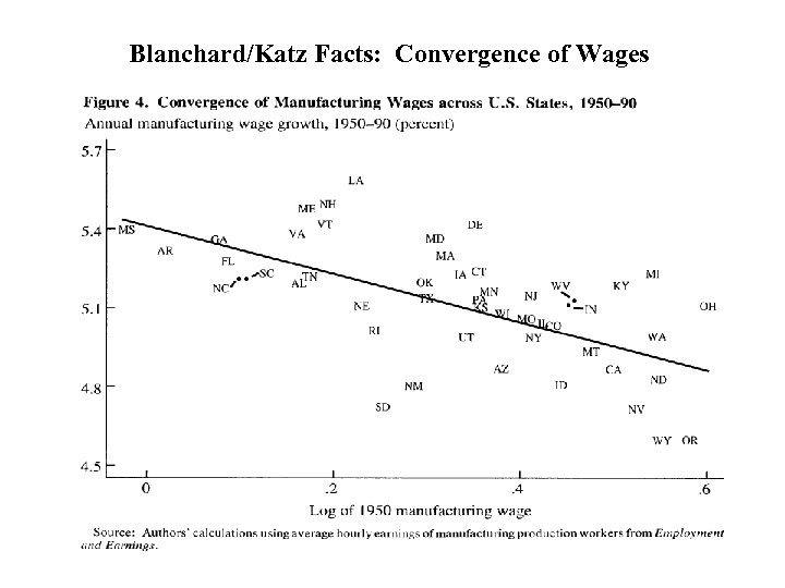 Blanchard/Katz Facts: Convergence of Wages
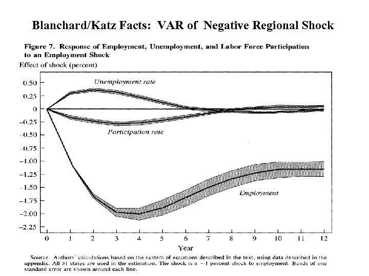 Blanchard/Katz Facts: VAR of Negative Regional Shock
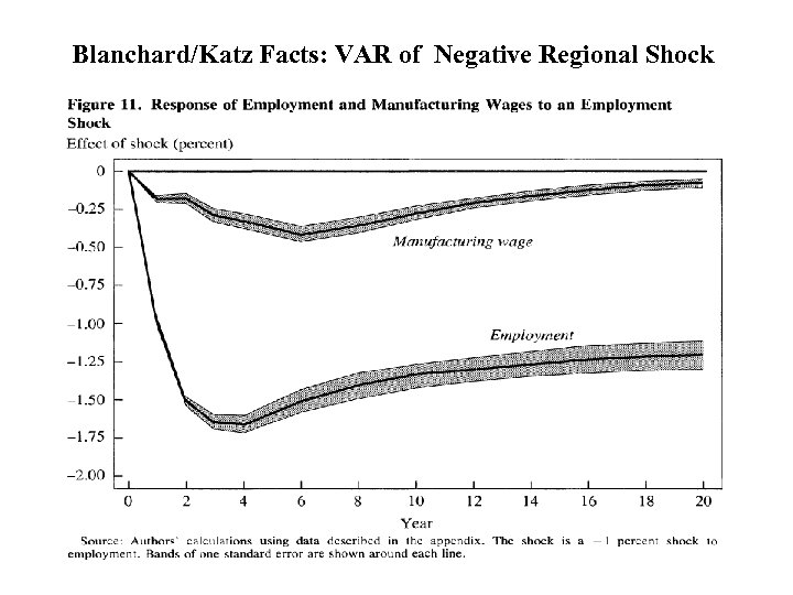 Blanchard/Katz Facts: VAR of Negative Regional Shock
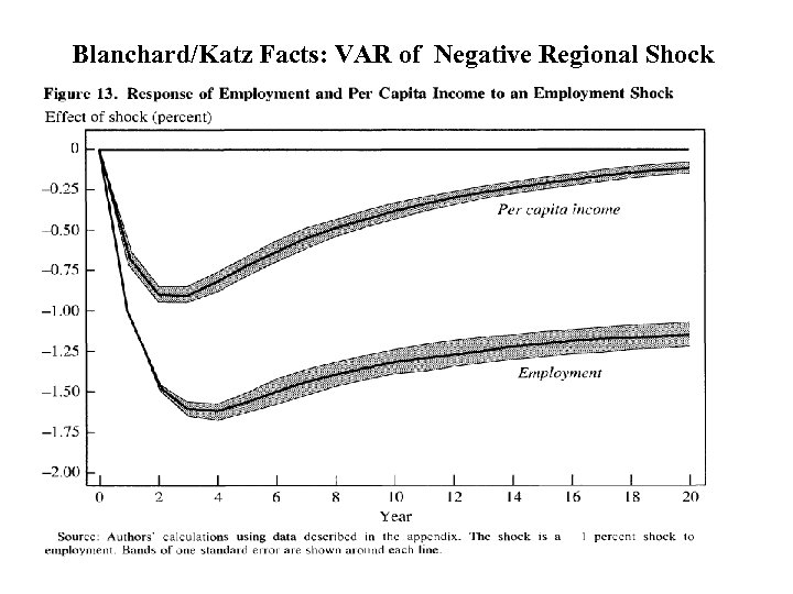 Blanchard/Katz Facts: VAR of Negative Regional Shock
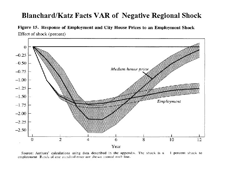 Blanchard/Katz Facts VAR of Negative Regional Shock
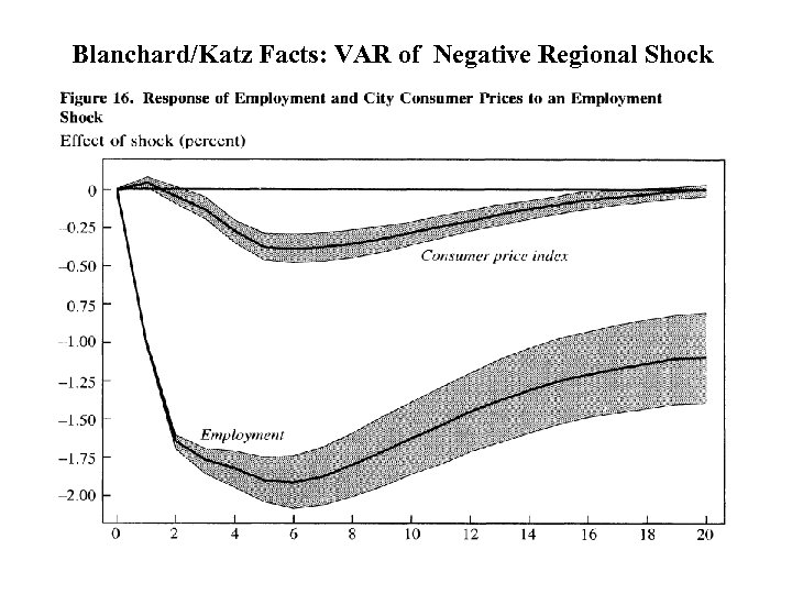 Blanchard/Katz Facts: VAR of Negative Regional Shock
 Conclusions of Blanchard/Katz • Regional Adjustments Take Place • In short run, response occurs on unemployment and wage margins. • In long run, it occurs on labor supply margin (via migration). • Spatial equilibrium model has to make individuals indifferent to move across regions.
 Part E: Regional Convergence (Barro and Sali-Martin)
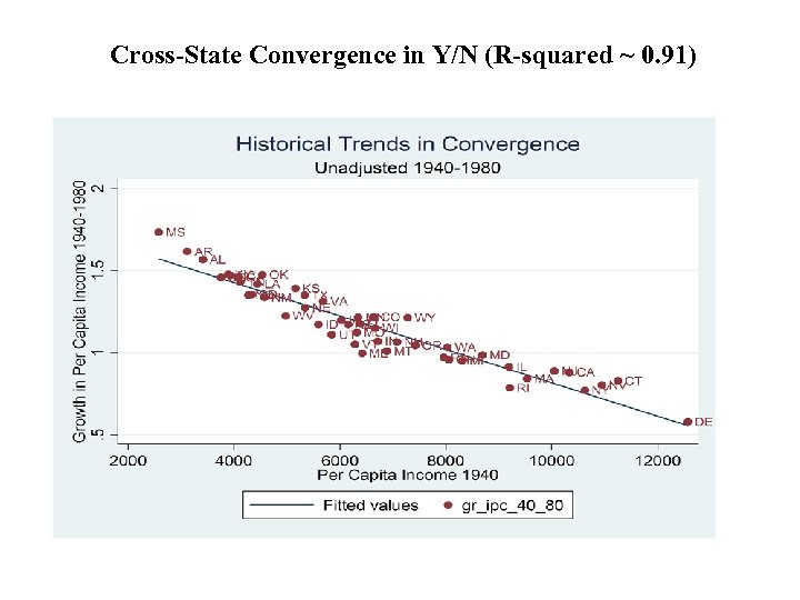 Cross-State Convergence in Y/N (R-squared ~ 0. 91)
 Part F: Recent Literature Using Regional Variation for Macro Questions
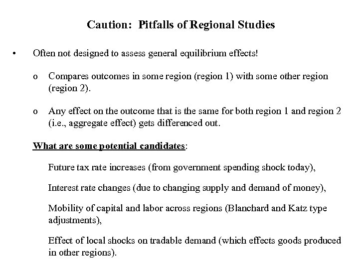 Caution: Pitfalls of Regional Studies • Often not designed to assess general equilibrium effects! o Compares outcomes in some region (region 1) with some other region (region 2). o Any effect on the outcome that is the same for both region 1 and region 2 (i. e. , aggregate effect) gets differenced out. What are some potential candidates: Future tax rate increases (from government spending shock today), Interest rate changes (due to changing supply and demand of money), Mobility of capital and labor across regions (Blanchard and Katz type adjustments), Effect of local shocks on tradable demand (which effects goods produced in other regions).
 4 Recent Papers on Spatial Equilibrium o Nakamura and Steinsson o Yagan o Giannone (in capital theory tomorrow) o Beraja, Hurst and Ospina


