Topic 1 b Review of Producer Theory supply Review

Topic 1(b): Review of Producer Theory (supply) Review of Supply. • Three areas to cover on the supply side: i. Interpreting an individual producer’s supply curve ii. Measuring producer well-being using the supply curve iii. Deriving aggregate supply from individual supply 1

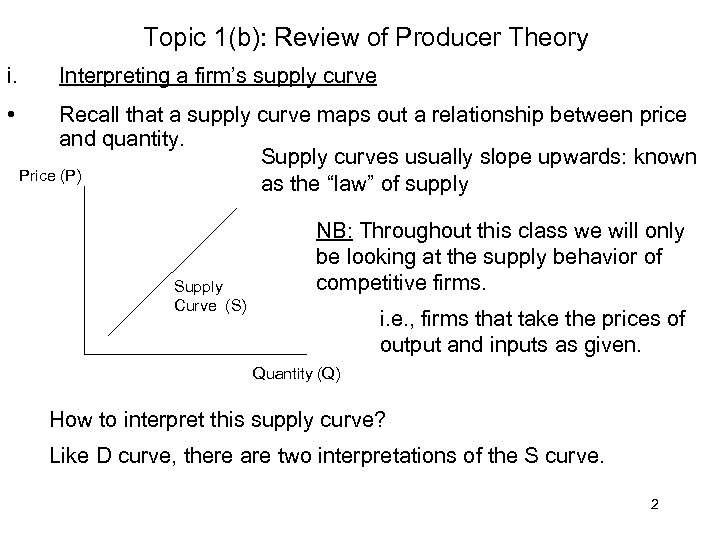
Topic 1(b): Review of Producer Theory i. • Interpreting a firm’s supply curve Recall that a supply curve maps out a relationship between price and quantity. Supply curves usually slope upwards: known Price (P) as the “law” of supply Supply Curve (S) NB: Throughout this class we will only be looking at the supply behavior of competitive firms. i. e. , firms that take the prices of output and inputs as given. Quantity (Q) How to interpret this supply curve? Like D curve, there are two interpretations of the S curve. 2

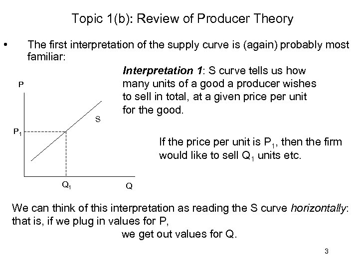
Topic 1(b): Review of Producer Theory • P The first interpretation of the supply curve is (again) probably most familiar: Interpretation 1: S curve tells us how many units of a good a producer wishes to sell in total, at a given price per unit for the good. S P 1 If the price per unit is P 1, then the firm would like to sell Q 1 units etc. Q 1 Q We can think of this interpretation as reading the S curve horizontally: that is, if we plug in values for P, we get out values for Q. 3

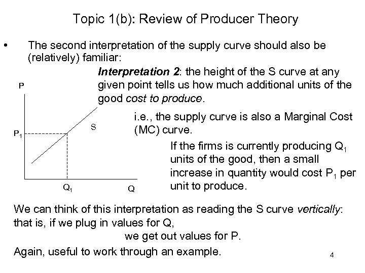
Topic 1(b): Review of Producer Theory • P The second interpretation of the supply curve should also be (relatively) familiar: Interpretation 2: the height of the S curve at any given point tells us how much additional units of the good cost to produce. S P 1 Q 1 i. e. , the supply curve is also a Marginal Cost (MC) curve. If the firms is currently producing Q 1 units of the good, then a small increase in quantity would cost P 1 per unit to produce. Q We can think of this interpretation as reading the S curve vertically: that is, if we plug in values for Q, we get out values for P. Again, useful to work through an example. 4

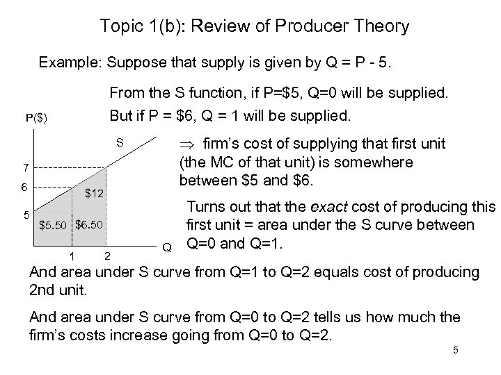
Topic 1(b): Review of Producer Theory Example: Suppose that supply is given by Q = P - 5. From the S function, if P=$5, Q=0 will be supplied. But if P = $6, Q = 1 will be supplied. P($) firm’s cost of supplying that first unit (the MC of that unit) is somewhere between $5 and $6. S 7 6 $12 5 $5. 50 $6. 50 1 2 Q Turns out that the exact cost of producing this first unit = area under the S curve between Q=0 and Q=1. And area under S curve from Q=1 to Q=2 equals cost of producing 2 nd unit. And area under S curve from Q=0 to Q=2 tells us how much the firm’s costs increase going from Q=0 to Q=2. 5

Topic 1(b): Review of Producer Theory • Area under S curve up to a given Q actually tells us the Variable Cost (VC) of producing that Q. • Recall that a firm’s Total Costs (TC) have 2 components: TC = Fixed Costs + Variable Costs = FC + VC. • By definition, FC don’t change as Q changes, while VC do. • So MC = TC/ Q = (FC+VC) / Q = VC / Q. • area under the S curve up to a given Q = MC of 1 st unit + MC of 2 nd unit + MC of third unit etc. • And adding up MCs is the same as calculating VC. 6

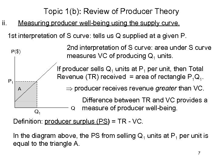
Topic 1(b): Review of Producer Theory ii. Measuring producer well-being using the supply curve. 1 st interpretation of S curve: tells us Q supplied at a given P. 2 nd interpretation of S curve: area under S curve measures VC of producing Q 1 units. P($) If producer sells Q 1 units at P 1 per unit, then Total Revenue (TR) received = area of rectangle P 1 Q 1. P 1 producer receives revenue greater than VC. A Q 1 Q Difference between TR and VC provides a measure of producer well-being. Definition: producer surplus (PS) = TR - VC. In the diagram above, the PS from selling Q 1 units at P 1 per unit is equal to the triangle A. 7

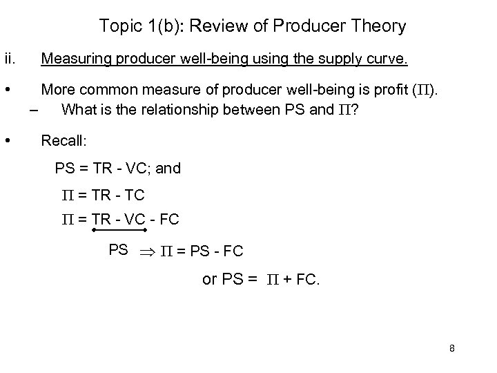
Topic 1(b): Review of Producer Theory ii. • • Measuring producer well-being using the supply curve. More common measure of producer well-being is profit ( ). – What is the relationship between PS and ? Recall: PS = TR - VC; and = TR - TC = TR - VC - FC PS = PS - FC or PS = + FC. 8

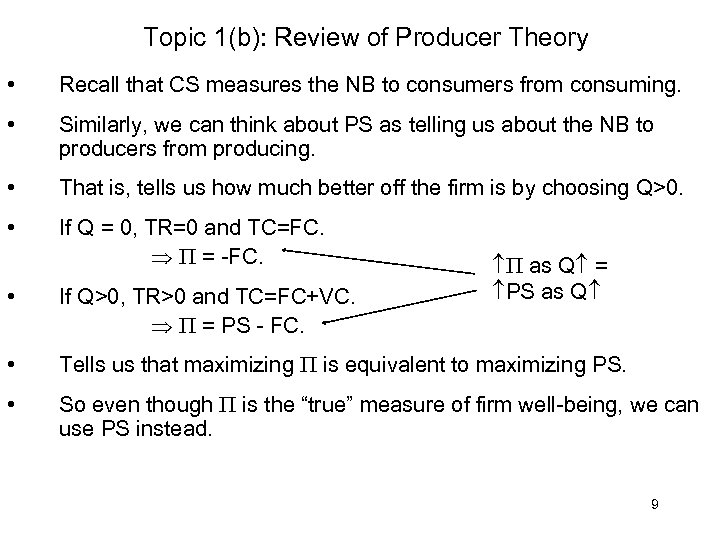
Topic 1(b): Review of Producer Theory • Recall that CS measures the NB to consumers from consuming. • Similarly, we can think about PS as telling us about the NB to producers from producing. • That is, tells us how much better off the firm is by choosing Q>0. • If Q = 0, TR=0 and TC=FC. = -FC. as Q = PS as Q • If Q>0, TR>0 and TC=FC+VC. = PS - FC. • Tells us that maximizing is equivalent to maximizing PS. • So even though is the “true” measure of firm well-being, we can use PS instead. 9

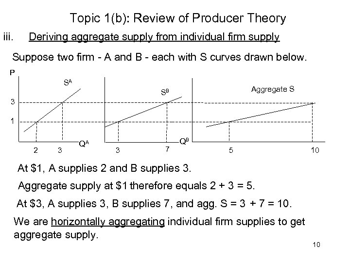
Topic 1(b): Review of Producer Theory iii. Deriving aggregate supply from individual firm supply Suppose two firm - A and B - each with S curves drawn below. P SA Aggregate S SB 3 1 2 3 QA 3 7 QB 5 10 At $1, A supplies 2 and B supplies 3. Aggregate supply at $1 therefore equals 2 + 3 = 5. At $3, A supplies 3, B supplies 7, and agg. S = 3 + 7 = 10. We are horizontally aggregating individual firm supplies to get aggregate supply. 10

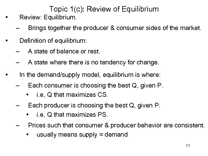
Topic 1(c): Review of Equilibrium • Review: Equilibrium. – • Brings together the producer & consumer sides of the market. Definition of equilibrium: – – • A state of balance or rest. A state where there is no tendency for change. In the demand/supply model, equilibrium is where: – Each consumer is choosing the best Q, given P. • i. e, Q that maximizes CS. – Each producer is choosing the best Q, given P. • i. e, Q that maximizes PS. – Prices such that consumer & producer behavior are consistent. • usually means supply = demand 11

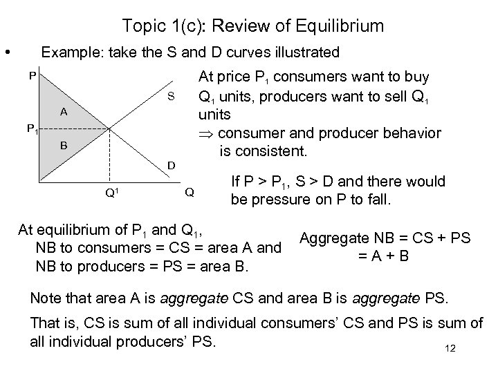
Topic 1(c): Review of Equilibrium • Example: take the S and D curves illustrated At price P 1 consumers want to buy Q 1 units, producers want to sell Q 1 units consumer and producer behavior is consistent. P S A P 1 B D Q 1 Q If P > P 1, S > D and there would be pressure on P to fall. At equilibrium of P 1 and Q 1, NB to consumers = CS = area A and NB to producers = PS = area B. Aggregate NB = CS + PS =A+B Note that area A is aggregate CS and area B is aggregate PS. That is, CS is sum of all individual consumers’ CS and PS is sum of all individual producers’ PS. 12

Topic 1(c): Review of Equilibrium Summary: • We have seen that : – Consumers choose Q such that P = MB • i. e. , choose to consume where P cuts D curve. • NB to consumers = CS. – Producers choose Q such that P = MC • i. e. choose to produce where P line cuts S curve. • NB to producers = PS. – Producer and consumer decisions are such that S=D • Aggregate NB = sum of individual NB • Sum of individual NB = CS + PS (if consumers and producers are the only agents affected by the market). 13