25792ae2e3a5a05094a0a41c5ee8280b.ppt
- Количество слайдов: 33
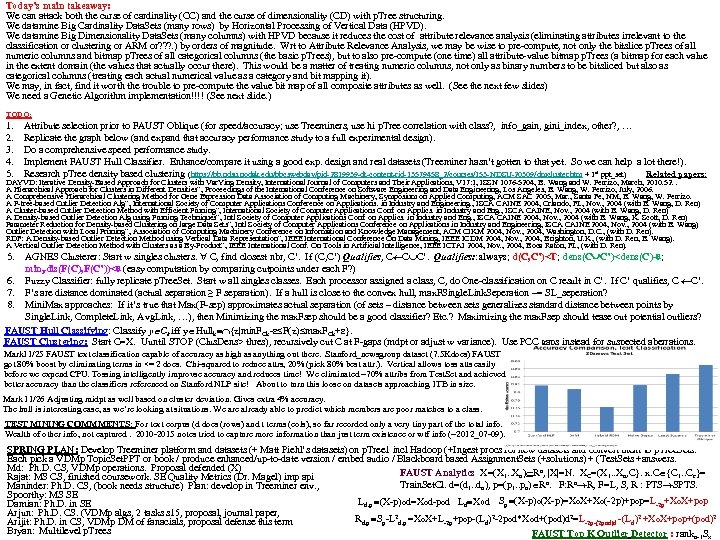
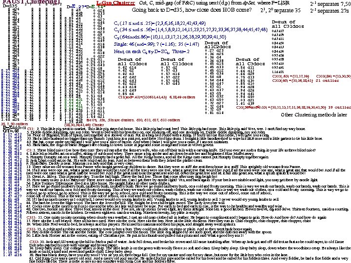
Today’s main takeaway: We can attack both the curse of cardinality (CC) and the curse of dimensionality (CD) with p. Tree structuring. We datamine Big Cardinality Data. Sets (many rows) by Horizontal Processing of Vertical Data (HPVD). We datamine Big Dimensionality Data. Sets (many columns) with HPVD because it reduces the cost of attribute relevance analysis (eliminating attributes irrelevant to the classification or clustering or ARM or? ? ? . ) by orders of magnitude. Wrt to Attribute Relevance Analysis, we may be wise to pre-compute, not only the bitslice p. Trees of all numeric columns and bitmap p. Trees of all categorical columns (the basic p. Trees), but to also pre-compute (one time) all attribute-value bitmap p. Trees (a bitmap for each value in the extent domain (the values that actually occur there). This would be a matter of treating numeric columns, not only as binary numbers to be bitsliced but also as categorical columns (treating each actual numerical value as a category and bit mapping it). We may, in fact, find it worth the trouble to pre-compute the value bit map of all composite attributes as well. (See the next few slides) We need a Genetic Algorithm implementation!!!! (See next slide. ) TODO: 1. 2. 3. 4. 5. Attribute selection prior to FAUST Oblique (for speed/accuracy; use Treeminers, use hi p. Tree correlation with class? , info_gain, gini_index, other? , … Replicate the graph below (and expand that accuracy performance study to a full experimental design). Do a comprehensive speed performance study. Implement FAUST Hull Classifier. Enhance/compare it using a good exp. design and real datasets (Treeminer hasn’t gotten to that yet. So we can help a lot there!). Research p. Tree density based clustering (https: //bb. ndsu. nodak. edu/bbcswebdav/pid-2819939 -dt-content-rid-13579458_2/courses/153 -NDSU-20309/dmcluster. htm + 1 st ppt_set) Related papers: DAYVD: Iterative Density-Based Approach for Clusters with Var. Ying Density, International Journal of Computers and Their Applications, V 17: 1, ISSN 1076 -5204, B. Wang and W. Perrizo, March, 2010. 52. . A Hierarchical Approach for Clusters in Different Densities”, Proceedings of the International Conference on Software Engineering and Data Engineering, Los Angeles, B. Wang, W. Perrizo, July, 2006. A Comprehensive Hierarchical Clustering Method for Gene Expression Data Association of Computing Machinery, Symposium on Applied Computing, ACM SAC 2005, Mar. , Santa Fe, NM, B. Wang, W. Perrizo. A P-tree-based Outlier Detection Alg”, International Society of Computer Applications Conference on Applications. in Industry and Engineering. , ISCA CAINE 2004, Orlando, FL, Nov. , 2004 (with B. Wang, D. Ren) A Cluster-based Outlier Detection Method with Efficient Pruning”, International Society of Computer Applications Conf. on Applics. in Industry and Eng. , ISCA CAINE, Nov. , 2004 (with B. Wang, D. Ren) A Density-based Outlier Detection Alg using Pruning Techniques”, Intl Society of Computer Applications Conf. on Applics. in Industry and Eng. , ISCA CAINE 2004, Nov. , 2004 (with B. Wang, K. Scott, D. Ren) Parameter Reduction for Density-based Clustering on large Data Sets”, Intl Society of Computer Applications Conference on Applications in Industry and Engineering, ISCA CAINE 2004, Nov. , 2004 (with B. Wang) Outlier Detection with Local Pruning”, Association of Computing Machinery Conference on Information and Knowledge Management, ACM CIKM 2004, Nov. , 2004, Washington, D. C. , (with D. Ren). RDF: A Density-based Outlier Detection Method using Vertical Data Representation”, IEEE International Conference On Data Mining, IEEE ICDM 2004, Nov. , 2004, Brighton, U. K. , (with D. Ren, B. Wang). A Vertical Outlier Detection Method with Clusters as a By-Product”, IEEE International Conf. On Tools in Artificial Intelligence, IEEE ICTAI 2004, Nov. , 2004, Boca Raton, FL, (with D. Ren). 5. AGNES Clusterer: Start w singles clusters. C, find closest nbr, C’. If (C, C’) Qualifies, C C C’. Qualifies: : always; d(C, C’)<T; dens(C C’)<dens(C)- ; min. Fdis(F(C), F(C’))< (easy computation by comparing cutpoints under each F? ) 6. Fuzzy Classifier: fully replicate p. Tree. Set. Start w all singles classes. Each processor assigned a class, C, do One-classification on C result in C’. If C’ qualifies, C C’. 7. F’s are distance dominated (actual separation ≥ F separation). If a hull is close to the convex hull, max. FSingle. Link. Seperation ~= SL_seperation? 8. Mini. Max approaches: If it’s true that Max(F-sep) approximates actual separation (of sets – distance between sets generalizes standard distance between points by Single. Link, Complete. Link, Avg. Link, …), then Minimizing the max. Fsep should be a good classifier? Etc. ? Maximizing the max. Fsep should tease out potential outliers? FAUST Hull Classifying: Classify y Ck iff y Hullk {z|min. FCk- F(z) max. FCk+ }. FAUST Clustering: Start C=X. Uuntil STOP (Clus. Dens> thres), recursively cut C at F-gaps (mdpt or adjust w variance). Use PCC gaps instead for suspected aberrations. Mark 11/25 FAUST text classification capable of accuracy as high as anything out there. Stanford_newsgroup dataset (7. 5 Kdocs) FAUST got 80% boost by eliminating terms in <= 2 docs. Chi-squared to reduce attrs, 20% (pick 80% best attr. ). Vertical allows toss atts easily before we expend CPU. Tossing intelligently improvse accuracy and reduces time! We eliminated ~70% attribs from Test. Set and achieved better accuracy than the classifiers referenced on Stanford NLP site! About to turn this loose on datasets approaching 1 TB in size. Mark 11/26 Adjusting midpt as well based on cluster deviation. Gives extra 4% accuracy. The hull is interesting case, as we’re looking at situations. We are already able to predict which members are poor matches to a class. TEST MINING COMMMENTS: For text corpus (d docs (rows) and t terms (cols), so far recorded only a very tiny part of the total info. Wealth of other info, not captured. 2010 -2015 notes tried to capture more information than just term existence or wtf info (~2012_07 -09). SPRING PLAN: Develop Treeminer platform and datasets (+ Matt Piehl’s datasets) on p. Tree 1 incl Hadoop (+Ingest procs for new datasets and convert them to p. Tree. Sets. Each pick a VDMp Topic. Set. PPT or book / produce enhanced/up-to-date version / embed audio / Blackboard based Assignment. Sets (+solutions) + (Test. Sets +answers. Md: Ph. D. CS, VDMp operations. Proposal defended (X) FAUST Analytics X=(X 1. . Xn) Rn, |X|=N. XC=(X 1. . Xn, C}. x. C {C 1. . Cc}= Rajat: MS CS, finished coursework. SE Quality Metrics (Dr. Magel) imp api Train. Set. Cl. d=(d 1. . dn), p=(p 1. . pn) Rn. F: Rn R, F=L, S, R : PTS SPTS. Maninder: Ph. D. CS, (book needs structure) Plan: develop in Treeminer env. , Spoorthy: MS SE Ld, p (X-p)od=Xod-pod Ld Xod Sp (X-p)o(X-p)=Xo. X+Xo(-2 p)+pop=L-2 p+Xo. X+pop Damian: Ph. D. in SE Arjun: Ph. D. CS. (VDMp algs, 2 tasks s 15, proposal, journal paper, Rd, p Sp-L 2 d, p =Xo. X+L-2 p+pop-(Ld)2 -2 pod*Xod+(pod)d 2=L-2 p-(2 pod)d -(Ld)2 +Xo. X+pop+(pod)2 Arijit: Ph. D. in CS, VDMp DM of fanacials, proposal defense this term Bryan: Multilevel p. Trees FAUST Top K Outlier Detector : rankn-1 Sx
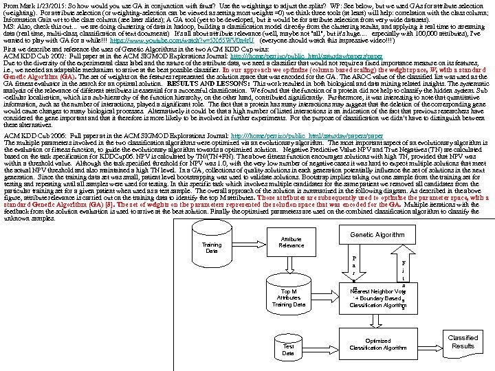
From Mark 1/23/2015: So how would you use GA in conjunction with faust? Use the weightings to adjust the splits? WP: See below, but we used GAs for attribute selection (weighting). For attribute selection (or weighting-selection can be viewed as setting most weights =0) we think three tools (at least) will help: correlation with the class column; Information Gain wrt to the class column (see later slides); A GA tool (yet to be developed, but it would be for attribute selection from very wide datasets). MS: Also, check this out. . . we are doing clustering of data in hadoop, building a classification model directly from the clustering results, and applying it real time to streaming data (real time, multi-class, classification of text documents) It's all about attribute relevance (well, maybe not "all", but it's huge. . especially with 100, 000 attributes), I've wanted to play with GA for a while!!! https: //www. youtube. com/watch? v=5 X 65 WV 0 n 4 r. U (everyone should watch this impressive video!!!) First we describe and reference the uses of Genetic Algorithms in the two ACM KDD Cup wins: ACM KDD Cub 2002: Full paper at in the ACM SIGMOD Explorations Journal: http: ///home/perrizo/public_html/saturday/papers/paper Due to the diversity of the experimental class label and the nature of the attribute data, we need a classifier that would not require a fixed importance measure on its features, i. e. , we needed an adaptable mechanism to arrive at the best possible classifier. In our approach we optimize (column based scaling) the weight space, W, with a standard Genetic Algorithm (GA). The set of weights on the features represented the solution space that was encoded for the GA. The AROC value of the classified list was used as the GA fitness evaluator in the search for an optimal solution. RESULTS AND LESSONS: This work resulted in both biological and data mining related insights. The systematic analysis of the relevance of different attributes is essential for a successful classification. We found that the function of a protein did not help to classify the hidden system. Sub -cellular localization, which is a sub-hierarchy of the function hierarchy, on the other hand, contributed significantly. Furthermore, it was interesting to note that quantitative information, such as the number of interactions, played a significant role. The fact that a protein has many interactions may suggest that the deletion of the corresponding gene would cause changes to many biological processes. Alternatively it could be that a high number of listed interactions is an indication of the fact that previous researchers have considered the gene important and that it therefore is more likely to be involved in further experiments. For the purpose of classification we didn’t have to distinguish between these alternatives. ACM KDD Cub 2006: Full paper at in the ACM SIGMOD Explorations Journal: http: ///home/perrizo/public_html/saturday/papers/paper The multiple parameters involved in the two classification algorithms were optimized via an evolutionary algorithm. The most important aspect of an evolutionary algorithm is the evaluation or fitness function, to guide the evolutionary algorithm towards a optimized solution. Negative Predictive Value NPV and True Negatives (TN) are calculated based on the task specification for KDDCup 06. NPV is calculated by TN/(TN+FN). The above fitness function encourages solutions with high TN, provided that NPV was within a threshold value. Although the task specified threshold for NPV was 1. 0, with the very low number of negative cases it was hard to expect multiple solutions that meet the actual NPV threshold and also maintained a high TN level. In a GA, collections of quality solutions in each generation potentially influence the set of solutions in the next generation. Since the training data set was small, patient level bootstrapping was used to validate solutions. Bootstrap implies taking out one sample from the training set for testing and repeating until all samples were used for testing. In this specific task which involves multiple candidates for the same patient we removed all candidates from the particular training set for a given patient when used as a test sample. The overall approach of the solution is summarized in the following diagram. As described in the above figure, attribute relevance is carried out on the training data to identify the top M attributes. Those attributes are subsequently used to optimize the parameter space, with a standard Genetic Algorithm (GA) [8]. The set of weights on the parameters represented the solution space that was encoded for the GA. Multiple iterations with the feedback from the solution evaluation is used to arrive at the best solution. Finally the optimized parameters are used on the combined classification algorithm to classify the unknown samples. Training Data Attribute Relevance Top M Attributes Training Data Test Data Genetic Algorithm P F a i r t a n m Nearest Neighbor Vote. + Boundary Based e s Classification Algorithm s Optimized Classification Algorithm Classified Results
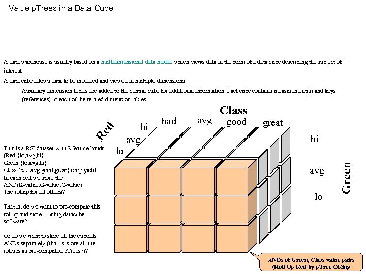
Value p. Trees in a Data Cube A data warehouse is usually based on a multidimensional data model which views data in the form of a data cube describing the subject of interest A data cube allows data to be modeled and viewed in multiple dimensions This is a RSI dataset with 2 feature bands (Red {lo, avg, hi} Green {lo, avg, hi} Class (bad, avg, good, great} crop yield In each cell we store the AND(R-value, G-value, C-value) The rollup for all others? lo hi avg bad avg Class good great hi avg lo Green Re d Auxiliary dimension tables are added to the central cube for additional information Fact cube contains measurement(s) and keys (references) to each of the related dimension tables. That is, do we want to pre-compute this rollup and store it using datacube software? Or do we want to store all the cuboids ANDs separately (that is, store all the rollups as pre-computed p. Trees? )? ANDs of Green, Class value pairs (Roll Up Red by p. Tree ORing
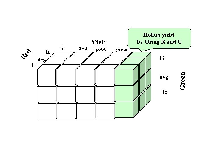
avg good great hi avg lo Green d Re lo hi avg lo Yield Rollup yield by Oring R and G
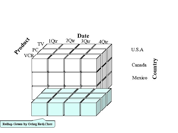
2 Qtr 3 Qtr 4 Qtr U. S. A Canada Mexico Rollup Green by Oring Red, Class Country t uc Pr od TV PC VCR 1 Qtr Date
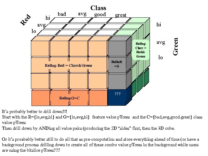
bad avg good great hi Rollup Class = Red& Green Rollup Red = Class&Green Rollup. G=C Rollu. R Rollup C=G =G avg lo Green d Re lo hi avg Class Rollup. C= R ? ? ? ? ? It’s probably better to drill down!!! Start with the R={lo, avg, hi} and G={lo, avg, hi} feature value p. Trees and the C={bad, avg, good. great} class value p. Trees Then drill down by ANDing all value pairs (producing the 2 D “sides” first, then the 3 D cube. Or it’s proabably better still to do all that as pre-computation and store everything ahead of time (or have a background process drilling down to create all of these combo value p. Trees in the background while users are using the bitslice p. Trees? ? ?
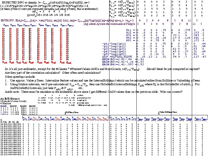
S 1, j= S 2, j= S 3, j= S 4, j= S 5, j= EXPECTED INFO to classify: I= - i=1. . m((rc. Pci)/|X|) log 2((rc. Pci)/|X|), m=5 I = -(3/16*log 3/16+1/4*log 1/4+1/8*log 1/8+3/16*log 3/16)= 2. 8 (If basic p. Tree rc’s are pre-computed (actually just value p. Trees), this is arithmetic!) rc. Pci = 3 4 4 2 3 pj=rc. Pci/16 = 3/16 1/4 1/8 3/16 rc(Pc=2^PBk=aj) rc(Pc=3^PBk=aj) rc(Pc=7^PBk=aj) rc(Pc=10^PBk=aj) rc(Pc=15^PBk=aj) 0 0 2 0 0 0 1 3 3 0 0 1 0 0 0 2 1 3 0 0 2 0 0 3 4 0 1 0 0 3 4 1 3 3 1 0 ENTROPY: E(Aj)= j=1. . v[(s 1 j+. . +smj)*I(s 1 j. . smj)/s] I(s 1 j. . smj)=- i=1. . m[pij*log 2(pij)] pij=sij/|Aj| sij=s 1, j+. . +s 5, j= 2 4 2 4 4 6 2 8 11 5 |Aj| where Aj's are the rootcounts of Pk(aj)'s 2 4 2 4 4 6 2 8 11 5 PB 2=3 PB 2=7 PB 2=10 PB 2=11 PB 3=4 B 3=5 PB 3=8 PB 4=11 P P P B 4=15 B 2=2 00 0 1 00 0 1 01 0 1 00 1 0 10 0 00 0 1 Pc=10 Pc=3 c=7 c=15 c=2 00 1 0 01 1 00 1 0 10 0 0 1 00 0 00 1 0 10 0 0 1 00 0 Pc=10 Pc=3 c=15 c=7 c=2 01 0 1 00 1 0 00 1 0 00 1 0 10 0 0 00 1 0 00 0 0 1 00 0 1 00 1 0 11 0 0 01 0 00 1 0 10 0 0 01 0 1 0 0 0 1 00 00 0 1 0 1 0 01 0 10 0 0 1 00 0 1 0 01 1 00 0 0 Pc=10 Pc=15 Pc=7 Pc=15 c=3 c=7 c=15 c=3 c=2 c=2 0 00 1 0 11 0 0 10 0 0 1 00 11 0 0 01 1 0 00 01 1 0 0 1 01 00 1 0 00 0 1 01 0 1 0 10 0 1 00 0 00 1 0 01 0 0 1 00 0 1 0 0 11 0 1 00 0 0 00 1 0 0 11 0 1 01 0 0 00 1 0 Pc=10 Pc=7 Pc=2 Pc=3 Pc=7 Pc=3 c=15 c=7 c=15 c=2 01 1 0 00 1 0 01 1 0 01 1 00 1 0 11 0 0 01 1 0 00 1 0 10 0 0 01 1 0 10 0 0 01 0 0 10 0 0 01 1 0 1 00 0 01 1 00 1 00 0 P 1 j = 0 0 0 P 2 j = 0. 5. 5 P 3 j = 1. 5 0 P 4 j = 0 0 0 P 5 j = 0 0 0 -p 1 j*log 2(p 1 j) 0. 5. 5 -p 2 j*log 2(p 2 j) 0. 5 0 -p 3 j*log 2(p 3 j) 0 0 0 -p 4 j*log 2(p 4 j) 0 0 0 -p 5 j*log 2(p 5 j) (s 1 j+. . +s 5 j)*I(s 1 j. . s 5 j)/16 0. 25. 13 GAIN(B 2)=2. 81 -. 89 =1. 92 GAIN(B 3)=2. 81 -1. 24 =1. 57 GAIN(B 4)=2. 81 -. 557 =2. 53 Pc=10 Pc=3 Pc=7 Pc=2 c=15 c=7 c=2 c=15 c=3 0 0 0. 25. 75 0 0 0. 5. 31. 2 . 75 0 0. 25 0. 75 0 0. 5 0. 31 0 0. 33. 17. 5 0 0. 52. 43. 5. 54 0 0 1 0 0 0 0 . 375. 5 0. 125 0. 53. 5 0. 37 0. 273. 363. 091. 273 0. 51. 53. 31. 51. 127 . 6. 2 0. 44. 46 0. 43 rc(PC=ci^PBk=aj). So it’s all just arithmetic, except for the #Classes * #Feature. Values ANDs and Root. Counts, Should these be pre-computed at capture? Are they part of the correlation calculation? Other often-used calculations? Other speedups include: 1. Use approx. Value p. Trees. Intervalize feature values and use the Interval. Bit. Maps (which can be calculated either from Bit. Slice or Value. Map p. Trees. 2. Using bitslice intervals, we’d pre-calculate all then use Hi. Order. Bit Interval. Bit. Maps, Pi, j, Kj where Kj is the Hi. Order. Bit of attrib, j. For Pi, j, k = PC=ci^Pj, k 2 nd. Hi. Order. Bit Intervals, just take Pi, j, Kj & P i, j, Kj-1 etc. Aside note: There must be mistakes in the arithmetic above since I get different GAIN values than on the previous slide. Who can correct? 3 0. 1875 -2. 4150 -0. 4528 An RSI Dataset 16 pixels (4 rows 4 cols): 4 bitslices 4 0. 25 -2 -0. 5 Band B 1: Band B 2: Band B 3: Band B 4: 3 3 7 7 7 3 3 2 8 8 4 5 11 15 11 11 3 3 7 7 7 3 3 2 8 8 4 5 11 11 2 2 10 15 11 11 10 10 8 8 4 4 15 15 11 11 2 10 15 15 11 11 10 10 8 8 4 4 15 15 11 11 4 2 3 0. 25 0. 187 -2 -3 -2. 41 -0. 5 -0. 37 -0. 45 2. 280 rc. Pci pi=rc. Pci/16 log 2(pi) pilog 2(pi) -SUM(pilog 2(pi)=I(c 1. . cm) Value Bit. Map p. Trees Bit. Slice p. Trees P 1, 3 P 1, 2 P 1, 1 P 1, 0 rc=5 S: X-Y B 1 B 2 B 3 B 4 0, 0 0011 0111 1000 1011 0 0, 1 0011 1000 1111 0 0, 2 0111 0011 0100 1011 0 0, 3 0111 0010 0101 1011 0 1, 0 0011 0111 1000 1011 0 1, 1 0011 1000 1011 0 1, 2 0111 0011 0100 1011 0 1, 3 0111 0010 0101 1011 0 2, 0 0010 1011 1000 1111 0 2, 1 0010 1011 1000 1111 0 2, 2 1010 0100 1011 1 2, 3 1111 1010 0100 1011 1 3, 0 0010 1011 1000 1111 0 3, 1 1010 1011 1000 1111 1 3, 2 1111 1010 0100 1011 1 3, 3 1111 1010 0100 1011. 1 Pc=2 Pc=3 Pc=7 Pc=10 Pc=15 P 2, 3 P 2, 2 P 2, 1 P 2, 0 P 3, 3 P 3, 2 P 3, 1 P 3, 0 P 4, 3 P 4, 2 P 4, 1 P 4, 0 P PB 2=3 PB 2=7 PB 2=10 PB 2=11 PB 3=4 B 3=5 PB 3=8 PB 4=11 B 4=15 P rc=7 rc=16 rc=11 rc=8 rc=2 rc=16 rc=10 rc=8 rc=0 rc=2 rc=16 rc=5 rc=16 rc=3 rc=4 rc=2 rc=3 PB 2=2 rc=4 rc=6 rc=2 rc=8 rc=11 rc=5 rc=2 0 0 1 1 0 0 0 1 1 1 1 1 1 1 0 0 0 1 1 0 0 0 0 1 1 1 1 1 0 0 0 0 1 1 1 1 1 0 1 1 0 0 1 1 0 0 1 1 0 0 0 0 0 0 1 0 0 0 0 0 1 1 1 1 0 1 0 0 0 1 1 1 1 1 1 1 1 1 0 0 0 0 1 1 0 0 1 1 0 0 0 0 0 0 0 0 1 0 0 0 0 1 0 0 1 1 0 0 0 0 0 1 1 0 0 0 0 0 0 0 0 0 1 1 0 0 0 0 1 0 0 0 1 0 0 0 0 1 1 0 0 1 0 1 1 1 0 0 1 1 0 1 0 0 0 1 1 0 0
Access to Ptree 1 and Ptree 2 William Perrizo To all my students (plus 3 former students who may be interested in an opportunity to use a p. Tree environment replete with massive, real-life big datasets that was developed by Treeminer Inc (the company that licensed p. Tree patents and is becoming a strong player in the vertical data mining area). The only requirement from this side is your willingness to share and willingness to sign a Treeminer NDA. I particularly am interested in having available for everyone to use a Genetic Algorithm tool. As we all know, Dr. Amal Shehan Perera was the lead scientist implementing a GA tool in p. Tree data mining software and it helped to win two ACM KDD Cups!!! Since that time my suggestion to anyone has been "When your done getting all you can out of your algorithm, GA it!!!" Baoying (Elizabeth)Wang did some amazing work on p. Tree clustering (and classification and ARM) and Dr. Imad Rahal did amazing p. Tree work on classification (and ARM and Clustering). That's why I invite Amal, Elizabeth and Imad to use our system once it gets up and going. My hope is that they will be willing to let us use any tools they develop in that system? ; -) (synergism). There may be other former Data. SURG members who would be interested as well (please advise). Just to update Amal, Elizabeth and Imad, Treeminer is a startup that has implemented a p. Tree data mining system in Java (about 70. 000 lines of code). It is wonderful and is commercially successful. Treeminer has used several Big. Data real-life dataset (captured in p. Trees). They have demonstrated both orders of magnitude improvement in speed (which is the traditional focus of p. Tree technology - speedup through Horizontal Processing of Vertical Data or HPVD) but also improvements in accuracy at the same time! This is unheard of and wonderful. Maybe the main reason we are able to get accuracy improvements while getting great speedup is that vertical structuring facilitates fast and effective attribute selection (which might take forever with horizontal data and therefore is not attempted in the horizontal data world). E. g. , when datamining a text corpus of 100, 000 vocab words (the columns) and 1 oo, 000 documents (the rows). it is important to find out the important words (attribute selection) before running an algorithm (solve the curse of dimensionality first). Amal, Elizabeth and Imad, if you would like to get involved, let us know. We still have Saturday meetings at 10 CST and we have two people who skype in every week (the more the merrier!). Arjun Roy or Arijit Chatterjee can tell how to skype in. Nathan Olson is our department technician who has helped us a lot. At this point we are nearly done getting all of Treeminer's stuff to the two p. Tree 1 and p. Tree 2 servers two servers, so that you can remote login to add anything to the GIT repository there (and run and test it against a very impressive suite of datasets. ) Please note I have posted all recent Saturday notes and other good materials on my web site: http: //www. cs. ndsu. nodak. edu/~perrizo You can get these materials by clicking on dot or period to the right of the bullet "media coverage" William Perrizo: I have put all the Saturday notes for the past few years and many other useful files (e. g. , topic synopses) on my web site so you all can access anything you want. I'm not worried at all about security since, if someone outside our group were to think they had stolen something important from there, then they probably would study it and become a p. Tree data mining expert. How could that be bad? You can get these materials by clicking on dot or period to the right of the bullet "media coverage" My homepage is: http: //www. cs. ndsu. nodak. edu/~perrizo There was a time in the past when I contemplated a "p. Tree Data Mining" monograph. I will put the very rough preliminary version of that book project on the website also. Anyone at all that every wants to co-author such a thing with me is welcome to work on it using the material at the site. I just wanted to ask if the 4 experience students (Damian, Mohammad, Arjun and Arijit) would be willing to help the students who will/may join our group (manider, Rajat, Spoorthy) and who will then be tasked to do coding, implementation and testing using Treeminer Software Environment and using Treeminer big vertical data sets? That would be great and would also help each of you, I believe. I'm sure Mark, Puneet will help also but they are, no doubt, buried under the weight of other needs right now. From: Bryan Mesich bryan. mesich@ndsu. edu Sent: Friday, January 23, 2015 12: 41 PM > I had the same question. We can make changes to code on ptree 1/2 directly but it will be difficult via VI editor. 2 relevant options. Take a copy in your local system, make changes and move the java file to ptree 1/2. Compile and run. > 2. Take a copy in your local system, make changes and compile. Move class file to ptree 1/2 and run. I do all of my development (Perl, C/C++. Assembly, Java, Bash) using VIM. This is my preference. I'm not advocating to use one IDE/Editor over another as its a personal choice. The best way to accomplish this would be to use a version system. That way you can do development on a remote machine and commit your changes. You could then log into ptree[12]. ndsu, checkout the latest version and run the code. Version control works well in collaborations efforts when merging code together. Also, I went ahead and installed both Java 7 and Java 8 JDKs on both servers. They are located in /usr/java. By default, Java 8 will be used when running/compiling. Bryan So we have any other alternatives I would suggest running GIT or SVN. Rajat > From: Arjun Roy > My IP address is 192. 168. 0. 4 > If for some reason I am not able to copy, Damian can give a try on campus? > I think the way we are going to proceed is that we will have Eclipse software on our client machine (pointing to code on ptree 1) but its going to be compiled on ptree 1. > I don't know if we can directly make changes to code stored on ptree 1 or if we would have to make changes locally and push it to ptree 1. > I dont have much knowledge on Java environment/Eclipse but does this sound logical (Rajat/Maninder)? > Thanks, Arjun > > From: Bryan Mesich <bryan. mesich@ndsu. edu> > Please give me a remote access. Once I have access, will put everything on Share. > > I have used it with Jdk 7 without any compiler complaints. > I need your IP address in order to make the exception in the firewall. > Also, did you use Open. JDK, or the official JDK from Oracle? > > Subject: Re: Access to Ptree 1 and Ptree 2 > > Logins are ready for use. I will be installing a firewall shortly > > that will only allow on-campus access. If you need remote access, > > please let me know and I'll make an exception for you in the firewall. > > Otherwise I'll assume everyone has access unless contacted. > > > Bryan, I have a few months old version of Tree. Miner. Its about 2. 5 GB. Is > > > it ok if I put the entire thing in my space on ptree 1 (might take a while to transfer)? > > Lets have you put the Tree. Miner code under the Shared directory > > (/stggroups/perrizo/Shared). That way everyone will have access to the code. > > > For latest version, we will have to contact Mark and go through some layers of security. > > We'll want to investigate a way to pull the code in an automated > > fashion in the future. The current version(s) you have should work for now. > > Does anyone know what JDK version Tree. Miner is using?
Damian Lampl Fri 1/23/2015 2: 12 PM I'll need remote access, too. My IP is: 208. 107. 126. 159 One reason we wanted to get things centralized on the p. Tree servers was so we wouldn't have to configure everyone's development environment separately (Java, Eclipse dependencies, etc) since that's the primary hang-up to getting started with the Treeminer code. I was thinking we could just remote desktop into the ptree servers using xrdp or something similar if that works? I really don't know the best way of setting it up so we all have access to the same preconfigured Java/Eclipse environment (. NET and Visual Studio would be a different story: install Visual Studio, done). You mentioned maven, Bryan, but I'm not familiar with how that works? Or if there's a configuration file we can get set up that makes sure our local Java, Eclipse, and any other dependencies are configured properly? I agree on a git repository so we'll have one main trunk and then separate branches for everyone, and when we need to merge with Mark's code, we can use the main trunk for that since he's also using git. Mark also has things working with Hadoop and some of his datasets will be stored in that. Bryan Mesich <bryan. mesich@ndsu. edu> Fri 1/23/2015 12: 41 PM Rajat Singh wrote: had the same question. > We can make changes to code on ptree 1/2 directly but it will be difficult via VI editor. So we have two relevant options > 1. Take a copy in your local system, make changes and move the java file to ptree 1/2. Compile and run. > 2. Take a copy in your local system, make changes and compile. Move class file to ptree 1/2 and run. I do all of my development (Perl, C/C++. Assembly, Java, Bash) using VIM. This is my preference. I'm not advocating to use one IDE/Editor over another as its a personal choice. The best way to accomplish this would be to use a version control system. That way you can do development on a remote machine and commit your changes. You could then log into ptree[12]. ndsu, checkout thel atest version and run code. Version control works well in collaborative efforts when merging code together. Also, I went ahead and installed both Java 7 and Java 8 JDKs on both servers. They are located in /usr/java. By default, Java 8 will be used when running/compiling. Bryan Maninder Singh Fri 1/23/2015 12: 21 PM Just a thought, can we think of some way to write a batch file in VI editor to do some of our work directly on ptree? Rajat Singh Fri 1/23/2015 12: 15 PM I had the same question. We can make changes to code on ptree 1/2 directly but it will be difficult via VI editor. So we have two relevant options 1. Take a copy in your local system, make changes and move the java file to ptree 1/2. Compile and run. 2. Take Arjun Roy Fri 1/23/2015 12: 08 PM My IP address is 192. 168. 0. 4 If for some reason I am not able to copy, Damian can give a try on campus? I think the way we are going to proceed is that we will have Eclipse software on our client machine (pointing to code on ptree 1) but its going to be compiled on ptree 1. I don't know if we can directly make changes to code stored on ptree 1 or if we would have to make changes locally and push it to ptree 1. I dont have much knowledge on Java environment/Eclipse but does this sound logical (Rajat/Maninder)? Arjun In my opinion, you can stay back at home and relax this Saturday : ) We students will collectively make it operational now that Bryan has created login for us. Logins are ready for use. I will be installing a firewall shortly that will only allow on-campus access. If you need remote access, please let me know and I'll make an exception for you in the firewall. Otherwise I'll assume everyone has access unless contacted. > > Bryan, I have a few months old version of Tree. Miner. Its about 2. 5 GB. Is > it ok if I put the entire thing in my space on ptree 1 (might take a while > to transfer)? Lets have you put the Tree. Miner code under the Shared directory (/stggroups/perrizo/Shared). That way everyone will have access to the code. > For latest version, we will have to contact Mark and go through some > layers of security. We'll want to investigate a way to pull the code in an automated fashion in the future. The current version(s) you have should work for now. Does anyone know what JDK version Tree. Miner is using?
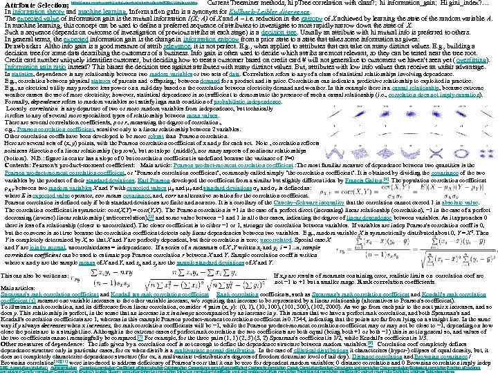
http: //www. cs. ndsu. nodak. edu/~perrizo/saturday/teach/879 s 15/dmlearn. htm Current Treeminer methods, hi p. Tree correlation with class? ; hi information_gain; Hi gini_index? … In information theory and machine learning, information gain is a synonym for Kullback–Leibler divergence. The expected value of information gain is the mutual information I(X; A) of X and A – i. e. reduction in the entropy of X achieved by learning the state of the random variable A. In machine learning, this concept can be used to define a preferred sequence of attributes to investigate to most rapidly narrow down the state of X. Such a sequence (depends on outcome of investigation of previous attribs at each stage) is a decision tree. Usually an attribute with hi mutual info is preferred to others. In general terms, the expected information gain is the change in information entropy from a prior state to a state that takes some information as given: Drawbacks: Altho info gain is a good measure of attrib relevance, it is not perfect. E. g. , when applied to attributes that can take on many distinct values. E. g. , building a decision tree for some data describing the customers of a business. Info gain is often used to decide which attribs are most relevant, so they can be tested near the tree root. Credit card number uniquely identifies customer, but deciding how to treat a customer based on credit card # will not generalize to customers we haven't seen yet ( overfitting). Information gain ratio instead? This biases the decision tree against attributes with many distinct values. But, attributes with low info values then receive an unfair advantage. Attribute Selection; In statistics, dependence is any relationship between two random variables or two sets of data. Correlation refers to any of a class of statistical relationships involving dependence. E. g. , correlation between physical statures of parents and offspring, ; between demand for a product and its price. Correlations can indicate a predictive relationship to exploited in practice. E. g. , an electrical utility may produce less power on a mild day based on the correlation between electricity demand weather. In this example there is a causal relationship, because extreme weather causes the use of more electricity; however, statistical dependence is not sufficient to demonstrate the presence of such a causal relationship (i. e. , correlation does not imply causation). Formally, dependence refers to random variables not satisfy inga math condition of probabilistic independence. Loosely correlation is any departure of two or more random variables from independence, but technically it refers to any of several more specialized types of relationship between mean values. There are several correlation coefficients, ρ or r, measuring the degree of correlation. , e. g. , Pearson correlation coefficient, sensitive only to a linear relationship between 2 variables. Other correlation coeffs have been developed to be more robust than Pearson correlation. Here are several sets of (x, y) points, with the Pearson correlation coefficient of x and y for each set. Note , correlation reflects noisiness /direction of a linear relationship (top row), but not slope (middle), nor many aspects of nonlinear relationships (bottom). N. B. : figure in center has a slope of 0 but correlation coefficient is undefined because the variance of Y=0 Contents: Pearson's product-moment coefficient: Main article: Pearson product-moment correlation coefficient : The most familiar measure of dependence between two quantities is the Pearson product-moment correlation coefficient, or "Pearson's correlation coefficient", commonly called simply "the correlation coefficient". It is obtained by dividing the covariance of the two variables by the product of their standard deviations. Karl Pearson developed the coefficient from a similar but slightly different idea by Francis Galton. [4] The population correlation coefficient ρX, Y between two random variables X and Y with expected values μX and μY and standard deviations σX and σY is defined as: where E is expected value operator, cov means covariance, and, corr an alternative notation for the correlation coefficient. Pearson correlation is defined only if both standard deviations are finite and nonzero. It is a corollary of the Cauchy–Schwarz inequality that the correlation cannot exceed 1 in absolute value. The correlation coefficient is symmetric: corr(X, Y) = corr(Y, X). The Pearson correlation is +1 in the case of a perfect direct (increasing) linear relationship (correlation), − 1 in the case of a perfect decreasing (inverse) linear relationship (anticorrelation), [5] and some value between − 1 and 1 in all other cases, indicating the degree of linear dependence between variables. As it approaches 0 there is less of a relationship (closer to uncorrelated). The closer coefficient is to either − 1 or 1, stronger the correlation between variables. If variables are indep Pearson's correlation coeff is 0, but the converse is not true because the correlation coefficient detects only linear dependencies between two variables. E. g. , random variable X is symmetrically distributed about 0, Y = X 2. Then Y is completely determined by X, so that X and Y are perfectly dependent, but their correlation is zero; uncorrelated. Special case X and Y are jointly normal, uncorrelatedness = independence. If a series of n measmnts of X , Y written xi and yi i = 1. . . n, sample correlation coefficient can be used to estimate pop Pearson correlation r between X and Y. Sample correlation coeff is written where x and y are the sample means of X and Y, and sx and sy are the sample standard deviations of X and Y. This can also be written as: If x, y are results of meamnts containing error, realistic limits on correlation coef are not − 1 to +1 but a smaller range. . Rank correlation coefficients Main articles: Spearman's rank correlation coefficient and Kendall tau rank correlation coefficient Rank correlation coefficients, such as Spearman's rank correlation coefficient and Kendall's rank correlation coefficient (τ) measure one variable increases to the other variable increase, w/o requiring that increase to be represented by a linear relationship (alternatives to Pearson's coefficient). To illustrate rank correlation, and its difference from linear correlation, consider 4 pairs (x, y): (0, 1), (10, 100), (101, 500), (102, 2000). As we go from each pair to the next pair x increases, and so does y. This relationship is perfect, in the sense that an increase in x is always accompanied by an increase in y. This means that we have a perfect rank correlation, and both Spearman's and Kendall's correlation coefficients are 1, whereas in this example Pearson product-moment correlation coefficient is 0. 7544, indicating that the points are far from lying on a straight line. In the same way if y always decreases when x increases, the rank correlation coefficients will be − 1, while the Pearson product-moment correlation coefficient may or may not be close to − 1, depending on how close the points are to a straight line. Although in the extreme cases of perfect rank correlation the two coefficients are both equal (being both +1 or both − 1) this is not in general so, and values of the two coefficients cannot meaningfully be compared. [7] For example, for the three pairs (1, 1) (2, 3) (3, 2) Spearman's coefficient is 1/2, while Kendall's coefficient is 1/3. Other measures of dependence: The info given by a correlation coef is not enough to define the dependence structure between random variables. [9] Correlation coef completely defines dependence structure only in particular cases, for ex when distrib is a multivariate normal distribution. In the case of elliptical distributions it characterizes (hyper-) ellipses of equal density, but, it does not completely characterize dependence structure (for ex, a multivariate t-distribution's degrees of freedom determine level of tail dep). Distance correlation and Brownian covariance / Brownian correlation[10][11] were introduced to address deficiency of Pearson's corr that it can be zero for dependent random variables; 0 distance correlation and 0 Brownian correlation imply indep SEE: Association (statistics) Autocorrelation Canonical correlation Coefficient of determination Cointegration Concordance correlation coefficient Cophenetic correlation Copula Correlation function Covariance and correlation Cross-correlation Ecological correlation Fraction of variance
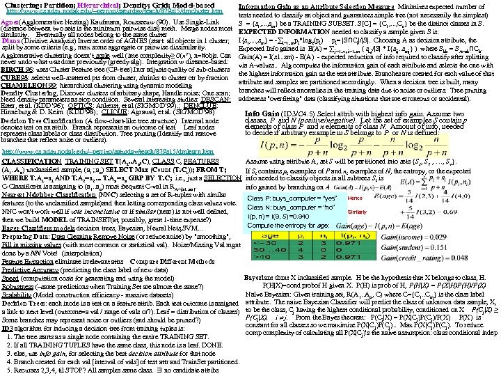
Clustering: Partition; Hierarchical; Density; Grid; Model-based http: //www. cs. ndsu. nodak. edu/~perrizo/saturday/teach/879 s 15/dmcluster. htm Agnes(Agglomerative Nesting) Kaufmann, Rousseeuw (90). Use Single-Link (distance between two sets is the minimum pairwise dist) meth. Merge nodes most similarity. Eventually all nodes belong to the same cluster Diana (Divisive Analysis) Inverse order of AGNES (start: all objects in 1 cluster; split by some criteria (e. g. , max some aggregate or pairwise dissimilarity. Agglomerative clustering doesn’t scale well (ime complexity≥O(n 2), n=#objs. Can never undo what was done previously (greedy alg). Integration w distance-based: BIRCH 96: uses Cluster Feature tree (CF-tree). Incr adjusts quality of sub-clusters CURE 98: selects well-scattered pts from cluster, shrinks to cluster ctr by fraction CHAMELEON 99: hierarchical clustering using dynamic modeling Density Clustering, Discover clusters of arbitrary shape, Handle noise; One scan; Need density parameters as stop condition. Several interesting studies: DBSCAN: Ester, et al. (KDD’ 96); OPTICS: Ankerst, et al (SIGMOD’ 99). ; DENCLUE: Hinneburg & D. Keim (KDD’ 98); CLIQUE: Agrawal, et al. (SIGMOD’ 98) Decision Tree Classification (A flow-chart-like tree structure) Internal node denotes test on an attrib. Branch represents an outcome of test. Leaf nodes represent class labels or class distribution. Tree pruning (Identify and remove branches that reflect noise or outliers). Information Gain as an Attribute Selection Measure Minimizes expected number of tests needed to classify an object and guarantees simple tree (not necessarily the simplest) S = {s 1, . . . , sm} be a TRAINING SUBSET. S[C] = {C 1, . . . , Cc} be the distinct classes in S. EXPECTED INFORMATION needed to classify a sample given S is: I{s 1, . . . , sm} = -∑i=1. . mpi*log 2(pi) pi= |S∩Ci|/|S|. Choosing A as decision attribute, the Expected Info gained is E(A) = ∑ j=1. . v; i=1. . m ( si, j/|S| * I{sij. . smj} ) where Skh = SA=ak∩Ch. Gain(A) = I(s 1. . sm) - E(A) - expected reduction of info required to classify after splitting via A-values. . Alg computes the information gain of each attribute and selects the one with the highest information gain as the test attribute. Branches are created for each value of that attribute and samples are partitioned accordingly. When a decision tree is built, many branches will reflect anomalies in the training data due to noise or outliers. Tree pruning addresess "overfitting" data (classifying situations that are erroneous or accidental). Info Gain (ID 3/C 4. 5) Select attrib with highest info gain. Assume two classes, P and N (positive/negative). Let the set of examples S contain p elements of class P and n elements of class N. Amount of info, needed to decide if arbitrary example in S belongs to P or N is defined: http: //www. cs. ndsu. nodak. edu/~perrizo/saturday/teach/879 s 15/dmlearn. htm Assume using attribute A, set S will be partitioned into sets {S 1, S 2 , …, Sv}. CLASSIFICATION TRAINING SET T(A 1. . An, C), CLASS C, FEATURES (A 1. . An) unclassified sample, (a 1; ; an) SELECT Max (Count (T. Ci)); FROM T; If Si contains pi examples of P and ni examples of N, the entropy, or the expected WHERE T. A 1=a 1 AND T. A 2=a 2. . . T. An=an GRP BY T. C; i. e. , just a SELECTION info needed to classify objects in all subtrees Si is C-Classificatn is assigning to (a 1. . an) most frequent C-val in RA=(a 1. . an). info gained by branching on A Nearest Neighbor Classification (NNC) selecting a set of R-tuples with similar Hence Class P: buys_computer = “yes” features (to the unclassified sample)and then letting corresponding class values vote. Class N: buys_computer = “no” NNC won't work well if vote inconclusive or if similar (near) is not well defined, Similarly I(p, n) = I(9, 5) =0. 940 then we build MODEL of TRAINSET(at, possibly, great 1 -time expense? ) Compute the entropy for age: Eager Classifiers models decision trees, Bayesian, Neural Nets, SVM. . . Preparing Data: Data Cleaning Remove Noise (or reduce noise) by "smoothing", Fill in missing values (with most common or statistical val). Noise/Missing Val mgnt done by a NN Vote! (interpolation) Feature Extraction eliminate irrelevant attrs Compare Different Methods Predictive Accuracy (predicting the class label of new data) Bayesian: thm: X inclassified sample. H be the hypothesis that X belongs to class, H. Speed (computation costs for generating and using the model) P(H|X)=cond probof H given X. P(H) is prob of H, P(H|X) = P(X|H)P(H)/P(X) Robustness (~same predictions when Training Set are almost the same? ) Naïve Bayesian: Given training set, R(A 1. . An, C) where C={C 1. . Cm} is the class label Scalability (Model construction efficiency - massive datasets) Decision Trees: each inode is a test on a feature attrib. Each test outcome is assigned attribute. The naive Bayesian Classifier will predict the class of unknown data sample, X, a link to next level (outcome=a val / range of vals or? ). Leaf = distribution of classes) to be the class, Cj having the highest conditional probability, conditioned on X P(Cj|X) ≥ P(Ci|X), i j. From the Bayes theorem: P(Cj|X) = P(X|Cj)P(Cj)/P(X) is Some branches may represent noise or outliers (and should be pruned? ) constant for all classes so we maximize P(X|C j)P(Cj). . Max P(X|Cj)P(Cj). To reduce ID 3 algorithm for inducing a decision tree from training tuples is: complexity of calculating all P(X|C j)'s the naive assumption: class conditional indep 1. The tree starts as a single node containing the entire TRAINING SET. 2. If all TRAINING TUPLES have the same class, this node is a leaf. DONE. 3. else, use info gain, for selecting the best decision attribute for that node 4. Branch created for each val [interval of vals] of test attr and Train. Set partitioned. 5. Recurses 2, 3, 4, til STOP? All samples same class. ∃ no candidate attribs

S 1, j= S 2, j= S 3, j= S 4, j= S 5, j= EXPECTED INFO to classify: I= - i=1. . m((rc. Pci)/|X|) log 2((rc. Pci)/|X|), m=5 I = -(3/16*log 3/16+1/4*log 1/4+1/8*log 1/8+3/16*log 3/16)= 2. 8 (If basic p. Tree rc’s are pre-computed (actually just value p. Trees), this is arithmetic!) rc. Pci = 3 4 4 2 3 pj=rc. Pci/16 = 3/16 1/4 1/8 3/16 rc(Pc=2^PBk=aj) rc(Pc=3^PBk=aj) rc(Pc=7^PBk=aj) rc(Pc=10^PBk=aj) rc(Pc=15^PBk=aj) 0 0 2 0 0 0 1 3 3 0 0 1 0 0 0 2 1 3 0 0 2 0 0 3 4 0 1 0 0 3 4 1 3 3 1 0 ENTROPY: E(Aj)= j=1. . v[(s 1 j+. . +smj)*I(s 1 j. . smj)/s] I(s 1 j. . smj)=- i=1. . m[pij*log 2(pij)] pij=sij/|Aj| sij=s 1, j+. . +s 5, j= 2 4 2 4 4 6 2 8 11 5 |Aj| where Aj's are the rootcounts of Pk(aj)'s 2 4 2 4 4 6 2 8 11 5 PB 2=3 PB 2=7 PB 2=10 PB 2=11 PB 3=4 B 3=5 PB 3=8 PB 4=11 P P P B 4=15 B 2=2 00 0 1 00 0 1 01 0 1 00 1 0 10 0 00 0 1 Pc=10 Pc=3 c=7 c=15 c=2 00 1 0 01 1 00 1 0 10 0 0 1 00 0 00 1 0 10 0 0 1 00 0 Pc=10 Pc=3 c=15 c=7 c=2 01 0 1 00 1 0 00 1 0 00 1 0 10 0 0 00 1 0 00 0 0 1 00 0 1 00 1 0 11 0 0 01 0 00 1 0 10 0 0 01 0 1 0 0 0 1 00 00 0 1 0 1 0 01 0 10 0 0 1 00 0 1 0 01 1 00 0 0 Pc=10 Pc=15 Pc=7 Pc=15 c=3 c=7 c=15 c=3 c=2 c=2 0 00 1 0 11 0 0 10 0 0 1 00 11 0 0 01 1 0 00 01 1 0 0 1 01 00 1 0 00 0 1 01 0 1 0 10 0 1 00 0 00 1 0 01 0 0 1 00 0 1 0 0 11 0 1 00 0 0 00 1 0 0 11 0 1 01 0 0 00 1 0 Pc=10 Pc=7 Pc=2 Pc=3 Pc=7 Pc=3 c=15 c=7 c=15 c=2 01 1 0 00 1 0 01 1 0 01 1 00 1 0 11 0 0 01 1 0 00 1 0 10 0 0 01 1 0 10 0 0 01 0 0 10 0 0 01 1 0 1 00 0 01 1 00 1 00 0 P 1 j = 0 0 0 P 2 j = 0. 5. 5 P 3 j = 1. 5 0 P 4 j = 0 0 0 P 5 j = 0 0 0 -p 1 j*log 2(p 1 j) 0. 5. 5 -p 2 j*log 2(p 2 j) 0. 5 0 -p 3 j*log 2(p 3 j) 0 0 0 -p 4 j*log 2(p 4 j) 0 0 0 -p 5 j*log 2(p 5 j) (s 1 j+. . +s 5 j)*I(s 1 j. . s 5 j)/16 0. 25. 13 GAIN(B 2)=2. 81 -. 89 =1. 92 GAIN(B 3)=2. 81 -1. 24 =1. 57 GAIN(B 4)=2. 81 -. 557 =2. 53 Pc=10 Pc=3 Pc=7 Pc=2 c=15 c=7 c=2 c=15 c=3 0 0 0. 25. 75 0 0 0. 5. 31. 2 . 75 0 0. 25 0. 75 0 0. 5 0. 31 0 0. 33. 17. 5 0 0. 52. 43. 5. 54 0 0 1 0 0 0 0 . 375. 5 0. 125 0. 53. 5 0. 37 0. 273. 363. 091. 273 0. 51. 53. 31. 51. 127 . 6. 2 0. 44. 46 0. 43 rc(PC=ci^PBk=aj). So it’s all just arithmetic, except for the #Classes * #Feature. Values ANDs and Root. Counts, Should these be pre-computed at capture? Are they part of the correlation calculation? Other often-used calculations? Other speedups include: 1. Use approx. Value p. Trees. Intervalize feature values and use the Interval. Bit. Maps (which can be calculated either from Bit. Slice or Value. Map p. Trees. 2. Using bitslice intervals, we’d pre-calculate all then use Hi. Order. Bit Interval. Bit. Maps, Pi, j, Kj where Kj is the Hi. Order. Bit of attrib, j. For Pi, j, k = PC=ci^Pj, k 2 nd. Hi. Order. Bit Intervals, just take Pi, j, Kj & P i, j, Kj-1 etc. Aside note: There must be mistakes in the arithmetic above since I get different GAIN values than on the previous slide. Who can correct? 3 0. 1875 -2. 4150 -0. 4528 An RSI Dataset 16 pixels (4 rows 4 cols): 4 bitslices 4 0. 25 -2 -0. 5 Band B 1: Band B 2: Band B 3: Band B 4: 3 3 7 7 7 3 3 2 8 8 4 5 11 15 11 11 3 3 7 7 7 3 3 2 8 8 4 5 11 11 2 2 10 15 11 11 10 10 8 8 4 4 15 15 11 11 2 10 15 15 11 11 10 10 8 8 4 4 15 15 11 11 4 2 3 0. 25 0. 187 -2 -3 -2. 41 -0. 5 -0. 37 -0. 45 2. 280 rc. Pci pi=rc. Pci/16 log 2(pi) pilog 2(pi) -SUM(pilog 2(pi)=I(c 1. . cm) Value Bit. Map p. Trees Bit. Slice p. Trees P 1, 3 P 1, 2 P 1, 1 P 1, 0 rc=5 S: X-Y B 1 B 2 B 3 B 4 0, 0 0011 0111 1000 1011 0 0, 1 0011 1000 1111 0 0, 2 0111 0011 0100 1011 0 0, 3 0111 0010 0101 1011 0 1, 0 0011 0111 1000 1011 0 1, 1 0011 1000 1011 0 1, 2 0111 0011 0100 1011 0 1, 3 0111 0010 0101 1011 0 2, 0 0010 1011 1000 1111 0 2, 1 0010 1011 1000 1111 0 2, 2 1010 0100 1011 1 2, 3 1111 1010 0100 1011 1 3, 0 0010 1011 1000 1111 0 3, 1 1010 1011 1000 1111 1 3, 2 1111 1010 0100 1011 1 3, 3 1111 1010 0100 1011. 1 Pc=2 Pc=3 Pc=7 Pc=10 Pc=15 P 2, 3 P 2, 2 P 2, 1 P 2, 0 P 3, 3 P 3, 2 P 3, 1 P 3, 0 P 4, 3 P 4, 2 P 4, 1 P 4, 0 P PB 2=3 PB 2=7 PB 2=10 PB 2=11 PB 3=4 B 3=5 PB 3=8 PB 4=11 B 4=15 P rc=7 rc=16 rc=11 rc=8 rc=2 rc=16 rc=10 rc=8 rc=0 rc=2 rc=16 rc=5 rc=16 rc=3 rc=4 rc=2 rc=3 PB 2=2 rc=4 rc=6 rc=2 rc=8 rc=11 rc=5 rc=2 0 0 1 1 0 0 0 1 1 1 1 1 1 1 0 0 0 1 1 0 0 0 0 1 1 1 1 1 0 0 0 0 1 1 1 1 1 0 1 1 0 0 1 1 0 0 1 1 0 0 0 0 0 0 1 0 0 0 0 0 1 1 1 1 0 1 0 0 0 1 1 1 1 1 1 1 1 1 0 0 0 0 1 1 0 0 1 1 0 0 0 0 0 0 0 0 1 0 0 0 0 1 0 0 1 1 0 0 0 0 0 1 1 0 0 0 0 0 0 0 0 0 1 1 0 0 0 0 1 0 0 0 1 0 0 0 0 1 1 0 0 1 0 1 1 1 0 0 1 1 0 1 0 0 0 1 1 0 0
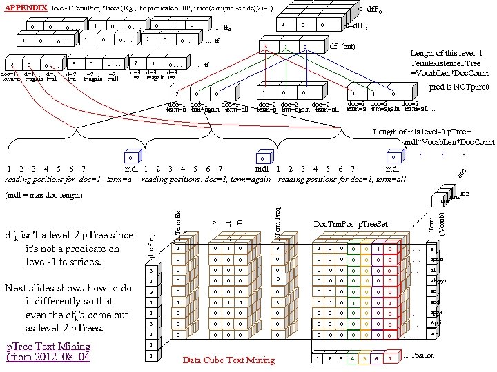
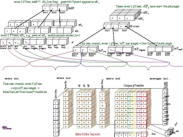
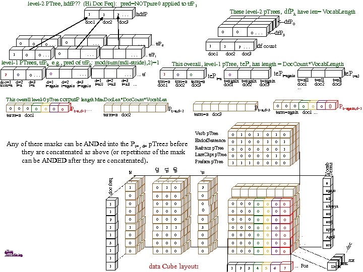
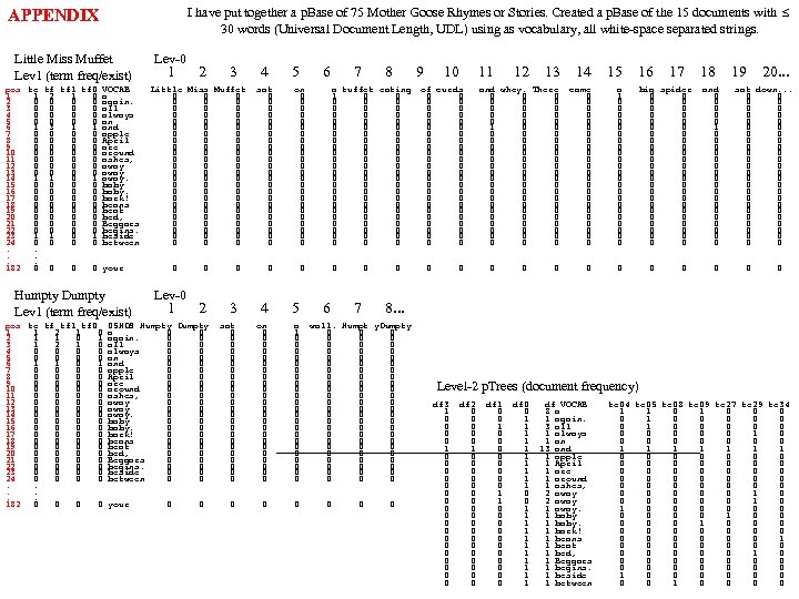
APPENDIX: level-1 Term. Freq. PTrees (E. g. , the predicate of tf. P 0: mod(sum(mdl-stride), 2)=1) 0 1 2 0 0 1 0 . . . doc=1 d=1 term=a t=again t=all 3 0. . . 0 0. . . d=2 t=again t=all 0 1 2 1 1 1 0. . . tf 0 0 0. . . tf 1 0. . . tf d=3 t=again t=all . . . 2 0 8 3 1 8 8 0 1 1 1 0 3 3 <--df. P 0 3 <--df. P 2 df (cnt) 0 Length of this level-1 Term. Existence. PTree =Vocab. Len*Doc. Count 1 0 0 0 1 1 pred is NOTpure 0 0 doc=3 doc=1 doc=2 term=a trm=again term=all. . . 0 Length of this level-0 p. Tree= mdl*Vocab. Len*Doc. Count . . . 0 0 . . . d oc 1 2 3 4 5 6 7 mdl reading-positions for doc=1, term=a reading-positions: doc=1, term=again reading-positions for doc=1, term=all JSE HHS LMM p. Tree Text Mining (from 2012_08_04 . . . tf 0 . . . Term Freq 1 0 2 1 0 0 1 0 . a 0 0 0 . again 0 0 0 . all 1 0 0 0 3 0 0 0 0 always. 2 0 0 0 an 1 1 0 1 1 3 0 1 0 0 1 and . . . Term (Vocab) . . . tf 1 0 . . doc freq . . . tf 2 Next slides shows how to do it differently so that even the dfk's come out as level-2 p. Trees. 1 3 dfk isn't a level-2 p. Tree since it's not a predicate on level-1 te strides. . Term Ex (mdl = max doc length) Doc. Trm. Pos p. Tree. Set 1 0 0 0 . . . apple 3 0 0 0 . April 1 0 0 0 . are 1 2 3 4 1 1 Data Cube Text Mining 5 6 7 . . . Position
level-2 PTree, hdf. P? ? (Hi Doc Feq): pred=NOTpure 0 applied to tf. P 1 1 These level-2 p. Trees, df. Pk have len= Vocab. Length hdf. P 0 . . . 1 doc 2 doc 3 0 0 1 0 0 . . . 0 . . . tf. P 0 1 . . . 8 8 8 0 1 1 1 3 3 3 0 . . . 2 . . . 1 <--df. P 0 <--df. P 3 df count doc 1 doc 2 doc 3 . . . tf. P 1 level-1 PTrees, tf. Pk e. g. , pred of tf. P 0: mod(sum(mdl-stride), 2)=1 0 0 . . . doc=1 d=2 d=3 term=a t=a 0 . . tf d=1 d=2 d=3 t=again t=all . . . This one, overall, level-1 p. Tree, te. P, has length = Doc. Count*Vocab. Length 1 0 0 trm=a term=a doc 1 doc 2 doc 3 te. Pt=a term=a doc 2 te. Pt=again te. Pt=all tr=all t=all doc 1 doc 2 doc 3 . . . t=again doc 1 doc 2 doc 3 term=a doc 3 . . . tf 0 . . . Term Freq 0 2 0 0 0 1 0 . . . 0 0 0 0 0 0 . . . 0 0 0 3 0 0 0 0 2 0 0 0 1 1 0 1 1 3 0 0 0 0 apple 1 0 0 0 . . . April 3 0 0 0 . are 1 0 0 0 . 1 2 3 4 Vocab Terms . . . tf 1 1 Corpus p. Tree. Set a data Cube layout: 5 6 7 all always. an and 1 1 again . . . Pos . . . doc freq 0 1 p. Tree Text Mining 1 1 This one, overall, level-0 p. Tree, corpus. P, has length = Max. Doc. Len*Doc. Count*Vocab. Len . . . tf 2 term=again doc 1. . . Term Ex term=a doc 1 0 oc 2 JSE HHS LMM
level-2 PTree, hdf. P? ? (Hi Doc Feq): pred=NOTpure 0 applied to tf. P 1 1 These level-2 p. Trees, df. Pk have len= Vocab. Length hdf. P 2 . . . 1 doc 2 doc 3 0 0 1 0 0 . . . 0 . . . tf. P 0 1 . . . doc=1 d=2 d=3 term=a t=a . . . 0 0 . . . tf d=1 d=2 d=3 t=again t=all . . . 8 8 0 1 1 1 3 3 0 . . . <--df. P 3 df count 2 . . . 1 <--df. P 0 3 doc 1 doc 2 doc 3 . . . tf. P 1 level-1 PTrees, tf. Pk e. g. , pred of tf. P 0: mod(sum(mdl-stride), 2)=1 2 8 This overall, level-1 p. Tree, te. P, has length = Doc. Count*Vocab. Length 1 0 0 te. Pt=a trm=a term=a doc 1 doc 2 doc 3 0 te. Pt=again t=again doc 1 doc 2 doc 3 te. Pt=al l tr=all t=all doc 1 doc 2 doc 3 . . . This overall level-0 p. Tree corpus. P length Max. Doc. Len*Doc. Count*Vocab. Len 0 term=a doc 1 0 0 Pt=a, d=1. . . Pt=a, d=2 term=a doc 3 0 1 0 0 0 Pt=again, d=1 0 1 0 0 0 1 1 1 0 0 1 0 2 0 0 0 1 0 0 0 . . . 1 0 0 0 3 0 0 0 0 2 0 0 0 1 1 0 1 1 3 0 0 0 0 apple 1 0 0 0 . . . April 3 0 0 0 . are 1 0 0 0 . 1 2 3 4 p. Tree Text Mining a again all an and 1 1 data Cube layout: 5 6 7 always. . Pos . . . doc freq . . . tf 0 0 . . . tf 0 1 0 . . . tf 1 0 0 . . . tf 2 Verb p. Tree Endof. Sentence Refrncs p. Tree Last. Chpt p. Tree Preface p. Tree 0 term=again doc 1. . . te Any of these masks can be ANDed into the Pt= , d= p. Trees before they are concatenated as above (or repetitions of the mask can be ANDED after they are concatenated). Pt=a, d=3 oc 0 Vocab Terms 0 JSE HHS LMM
I have put together a p. Base of 75 Mother Goose Rhymes or Stories. Created a p. Base of the 15 documents with 30 words (Universal Document Length, UDL) using as vocabulary, all white-space separated strings. APPENDIX Little Miss Muffet Lev 1 (term freq/exist) pos te tf tf 1 tf 0 VOCAB 1 1 2 1 0 a 2 0 0 again. 3 0 0 all 4 0 0 always 5 0 0 an 6 1 3 1 1 and 7 0 0 apple 8 0 0 April 9 0 0 are 10 0 0 around 11 0 0 ashes, 12 0 0 away 13 0 0 away 14 1 1 0 1 away. 15 0 0 baby 16 0 0 baby. 17 0 0 bark! 18 0 0 beans 19 0 0 beat 20 0 0 bed, 21 0 0 Beggars 22 0 0 begins. 23 1 1 0 1 beside 24 0 0 between. . . 182 0 0 your Humpty Dumpty Lev 1 (term freq/exist) pos te tf tf 1 tf 0 1 1 2 1 0 2 1 1 0 1 3 1 2 1 0 4 0 0 5 0 0 6 1 1 0 1 7 0 0 8 0 0 9 0 0 10 0 0 11 0 0 12 0 0 13 0 0 14 0 0 15 0 0 16 0 0 17 0 0 18 0 0 19 0 0 20 0 0 21 0 0 22 0 0 23 0 0 24 0 0. . . 182 0 0 Lev-0 1 2 3 4 5 6 7 8 9 10 11 12 13 14 15 16 17 18 19 20. . . Little Miss Muffet 0 0 0 0 0 0 0 0 0 0 0 0 0 0 0 0 0 0 0 on 0 0 0 0 0 0 0 a tuffet eating 1 0 0 0 0 0 0 0 0 0 0 0 0 0 0 0 0 0 0 0 of curds 0 0 0 0 0 0 0 0 0 0 0 0 0 and whey. There 0 0 0 0 1 0 0 0 0 0 0 0 0 0 0 0 0 0 0 0 came 0 0 0 0 0 0 a 1 0 0 0 0 0 0 big spider 0 0 0 0 0 0 0 0 0 0 0 0 0 and 0 0 0 1 0 0 0 0 0 sat down. . . 0 0 0 0 0 0 0 0 0 0 0 0 0 Lev-0 1 2 3 4 5 6 7 8. . . 05 HDS Humpty Dumpty a 0 0 again. 0 0 all 0 0 always 0 0 and 0 0 apple 0 0 April 0 0 are 0 0 around 0 0 ashes, 0 0 away. 0 0 baby. 0 0 bark! 0 0 beans 0 0 beat 0 0 bed, 0 0 Beggars 0 0 begins. 0 0 beside 0 0 between 0 0 your sat 0 0 0 0 0 0 0 sat 0 0 0 0 0 0 on 0 0 0 0 0 0 a 1 0 0 0 0 0 0 0 wall. Humpt y. Dumpty 0 0 0 0 0 0 0 0 0 0 0 0 0 0 0 0 0 0 0 Level-2 p. Trees (document frequency) df 3 1 0 0 0 0 0 0 df 2 0 0 0 1 0 0 0 0 0 df 1 0 0 0 0 0 1 1 0 0 0 df 0 0 1 1 1 1 1 1 df VOCAB 8 a 1 again. 3 all 1 always 1 an 13 and 1 apple 1 April 1 are 1 around 1 ashes, 2 away 1 away. 1 baby. 1 bark! 1 beans 1 beat 1 bed, 1 Beggars 1 begins. 1 beside 1 between te 04 te 05 te 08 te 09 te 27 te 29 te 34 1 1 0 0 0 0 0 0 0 1 0 0 0 0 1 1 1 1 0 0 0 0 0 0 0 0 0 0 1 0 0 0 0 0 0 1 0 0 0 0 0 0 0 0 1 0 0 0 0 1 0 0 0 0 1 0 0
FAUST 2^? 1 0 -1 -2 Clustering 1 D=d 35 L-Gap Clusterer Cut, C, mid-gap (of F&C) using next (d, p) from dp. Set, where F=L|S|R Cut, C, mid-gap (of F&C) using next (d, p) from dp. Set, D=. 27 s. D=. 64 s 2 -1 separates 7, 50 2 -2 separates. 27 s 0 d 26 0 0 0 d 9 0 d 26 Going back to D=d 35, how close does HOB come? 21, 20 separate 35 0 d 1 0 0 0 d 49 0 d 33 0 d 27 0 0 0 d 45 0 d 3 0 0 0. 09 d 6 0 d 44 0 0 0. 09 d 3 0 d 27 0 d 16 0 0 0 D=sum of 0 d 45 C 1 (. 17 xod . 25)={2, 3, 6, 18, 22, 43, 49} 0. 09 d 33 0 d 6 0 0 0 d 2 all C 31 docs 0 d 17 0 0 0. 09 d 18 0 d 44 0 d 47 0 0 0. 09 d 44 C 2 (. 34 xod . 56)={1, 4, 5, 8, 9, 12, 14, 15, 23, 25, 27, 32, 33, 36, 37, 38, 44, 45, 47, 48} 0. 63 d 17 0 d 23 0 d 18 0 0 0. 18 d 43 0 d 10 0 d 9 0. 63 d 29 0 0 0. 18 d 25 0 d 43 C 3 (. 64 xod. 86)={10, 11, 13, 17, 21, 26, 28, 29, 30, 39, 41, 50} 0 0 0. 18 d 22 0 d 15 0. 63 d 11 0 d 12 0 0 0. 18 d 12 0 d 49 0 d 33 0 0 0. 18 d 16 0. 84 d 50 0 d 16 Single: 46 (xod=. 99); 7 (=1. 16); 35 (=1. 47) D=sum of 0 d 14 0 0 0. 18 d 2 0 d 38 0. 84 d 13 all. C 2 docs 0 d 23 0 0 0. 27 d 27 0 d 6 0 d 49 0 0 0. 27 d 23 0. 84 d 30 Next, on each Ck try D= Ck, Thres=. 2 0 d 25 0 0 0 d 18 0. 36 d 25 0 d 45 0. 95 d 26 0 0 0. 27 d 42 0 d 22 0. 36 d 4 0 d 2 0 0 0. 27 d 15 0. 25 d 1 0. 95 d 28 D=sum of 0 d 29 0. 36 d 38 0 0 0. 27 d 13 0. 25 d 37 0 d 13 0 0 0. 27 d 47 0. 45 d 15 all C 1 docs all C 11 docs all C 3 docs 0. 95 d 10 0 d 9 0 0 0. 36 d 26 0. 25 d 43 0. 45 d 33 0. 42 d 16 0. 57 d 2 0. 56 d 11 0. 95 d 41 0 d 32 0. 25 d 8 0 0 0. 45 d 12 0. 27 d 28 0. 27 0 0 0 1 0. 36 d 29 0. 25 d 29 0. 42 d 2 0. 57 d 3 0. 66 d 17 1. 16 d 21 0. 27 d 41 0. 27 0 0 0 1 0. 36 d 36 0. 25 d 25 0. 45 d 36 0. 42 d 3 0. 57 d 16 0. 66 d 29 0. 46 d 38 0. 27 d 42 0. 27 0 0 0 1 0. 46 d 14 0. 25 d 42 C 311(. . 63) ={11, 17, 29} C 312(. 84) ={13, 30, 50} 0. 54 d 8 0. 42 d 42 0. 57 d 22 0. 75 d 13 0. 27 d 30 0. 27 0 0 0 1 0. 46 d 48 0. 54 d 44 0. 25 d 12 0. 42 d 43 0. 57 d 42 0. 85 d 30 C 313(. 95) ={10, 26, 28, 41} 21 outlier 0. 27 d 21 0. 27 0 0 0 1 0. 54 d 47 0. 27 d 22 0. 27 0 0 0 1 0. 46 d 8 0. 25 d 47 0. 42 d 22 0. 57 d 43 0. 85 d 10 0. 27 d 15 0. 27 0 0 0 1 0. 46 d 10 0. 25 d 48 0. 63 d 18 0. 94 d 28 0. 27 d 36 0. 27 0 0 0 1 0. 46 d 37 0. 51 d 32 0. 63 d 37 0. 63 d 49 0. 94 d 26 0. 27 d 11 0. 27 0 0 0 1 0. 55 d 32 0. 51 d 14 0. 63 d 5 0. 85 d 6 0. 94 d 41 0. 27 d 38 0. 27 0 0 0 1 0. 55 d 1 0. 51 d 4 0. 27 d 46 0. 27 0 0 0 1 0. 55 d 5 0. 63 d 32 0. 94 d 50 C 11(xod=. 42)={231622, 43} 6, 18, 49 outliers 0. 27 d 5 0. 27 0 0 0 1 0. 64 d 21 0. 51 d 36 0. 63 d 50 1. 03 d 21 0. 27 d 8 0. 27 0 0 0 1 0. 64 d 4 0. 51 d 13 0. 72 d 27 1. 41 d 39 0. 27 d 37 0. 27 0 0 0 1 0. 64 d 11 0. 51 d 5 0. 72 d 45 0. 27 d 48 0. 27 0 0 0 1 0. 64 d 17 0. 77 d 10 C 31(. 56 xod 1. 03) ={10, 11, 13, 17, 21, 26, 28, 29, 30, 41, 50} 39 outlier 0. 27 d 39 0. 27 0 0 0 1 0. 92 d 30 1. 03 d 11 0. 72 d 9 0. 27 d 4 0. 27 0 0 0 1 1. 01 d 41 1. 29 d 17 0. 81 d 14 0. 55 d 50 0. 55 0 0 1 0 Other Clustering methods later 0. 55 d 7 0. 55 0 0 1. 01 d 28 1. 54 d 21 3. 60 d 35 3. 60 1 1 1 0 1. 10 d 39 the 0's, . 25 s, . 51 s are clusters. d 10, d 11, d 17, d 21 outliers 1. 29 d 46 35, 7, 50 outliers {28, 30, 39, 41, 46} Cluster D= 44 docs C 11: 2. This little pig went to market. This little pig stayed at home. This little pig had roast beef. This little pig had none. This little pig said Wee, wee. I can't find my way home. GT=. 08 3. Diddle dumpling, my son John. Went to bed with his breeches on, one stocking off, and one stocking on. Diddle dumpling, my son John. 0. 17 d 22 16. Flour of England, fruit of Spain, met together in a shower of rain. Put in a bag tied round with a string. If you'll tell me this riddle, I will give you a ring. 0. 17 d 49 22. Had a little husband no bigger than my thumb. I put him in a pint pot, and there I bid him drum. I bought a little handkerchief to wipe his little nose and a little garters to tie his little hose. 0. 21 d 42 42. Bat bat, come under my hat and I will give you a slice of bacon. And when I bake I will give you a cake, if I am not mistaken. 0. 21 d 2 0. 21 d 16 43. Hark hark, the dogs do bark! Beggars are coming to town. Some in jags and some in rags and some in velvet gowns. 0. 25 d 18 C 2: 1. Three blind mice! See how they run! They all ran after the farmer's wife, who cut off their tails with a carving knife. Did you ever see such a thing in your life as three blind mice? 0. 25 d 3 0. 25 d 43 4. Little Miss Muffet sat on a tuffet, eating of curds and whey. There came a big spider and sat down beside her and frightened Miss Muffet away. 0. 25 d 6 5. Humpty Dumpty sat on a wall. Humpty Dumpty had a great fall. All the Kings horses, and all the Kings men cannot put Humpty Dumpty together again. 0. 34 d 23 8. Jack Sprat could eat no fat. His wife could eat no lean. And so between them both they licked the platter clean. 0. 34 d 15 9. Hush baby. Daddy is near. Mamma is a lady and that is very clear. 0. 34 d 44 12. There came an old woman from France who taught grown-up children to dance. But they were so stiff she sent them home in a sniff. This sprightly old woman from France. 0. 34 d 38 0. 34 d 25 14. If all seas were one sea, what a great sea that would be! And if all the trees were one tree, what a great tree that would be! And if all the axes were one axe, what a great axe that would be! And if all the 0. 34 d 36 men were one man what a great man he would be! And if the great man took the great axe and cut down the great tree and let it fall into great sea, what a splish splash it would be! 0. 38 d 33 15. Great A. little a. This is pancake day. Toss the ball high. Throw the ball low. Those that come after may sing heigh ho! 0. 38 d 48 23. How many miles is it to Babylon? Three score miles and ten. Can I get there by candle light? Yes, and back again. If your heels are nimble and light, you may get there by candle light. 0. 38 d 8 36. Little Tommy Tittlemouse lived in a little house. He caught fishes in other mens ditches. 0. 43 d 4 0. 43 d 12 37. Here we go round mulberry bush, mulberry bush. Here we go round mulberry bush, on a cold and frosty morning. This is way we wash our hands, wash our hands. This is 0. 47 d 47 way we wash our hands, on a cold and frosty morning. This is way we wash our clothes, wash our clothes. This is way we wash our clothes, on a cold and frosty morning. This is way we go to school, go to school. This is the way we go to school, on a cold and frosty morning. This is the way we come out of school, 0. 47 d 9 0. 47 d 37 come out of school. This is the way we come out of school, on a cold and frosty morning. 0. 51 d 5 38. If I had as much money as I could tell, I never would cry young lambs to sell. Young lambs to sell, young lambs to sell. I never would cry young lambs to sell. 0. 56 d 1 0. 56 d 32 44. The hart he loves the high wood. The hare she loves the hill. The Knight he loves his bright sword. The Lady loves her will. 0. 56 d 45 47. Cocks crow in the morn to tell us to rise and he who lies late will never be wise. For early to bed and early to rise, is the way to be healthy and wise. 0. 56 d 14 48. One two, buckle my shoe. Three four, knock at the door. Five six, ick up sticks. Seven eight, lay them straight. Nine ten. a good fat hen. Eleven twelve, dig and delve. Thirteen fourteen, maids a courting. 0. 56 d 27 Fifteen sixteen, maids in the kitchen. Seventeen eighteen. maids a waiting. Nineteen twenty, my plate is empty. 0. 64 d 10 0. 64 d 17 C 311: 11. One misty morning when cloudy was weather, I met an old man clothed all in leather. He began to compliment and I began to grin. How do And how do? And how do again 0. 64 d 21 17. Here sits the Lord Mayor. Here sit his two men. Here sits the cock. Here sits the hen. Here sit the little chickens. Here they run in. Chin chopper, chin! 0. 64 d 29 29. When little Fred went to bed, he always said his prayers. He kissed his mamma and then his papa, and straight away went upstairs. 0. 64 d 11 0. 69 d 26 C 312: 13. A robin and a robins son once went to town to buy a bun. They could not decide on plum or plain. And so they went back home again. 0. 69 d 50 30. Hey diddle! The cat and the fiddle. The cow jumped over the moon. The little dog laughed to see such sport, and the dish ran away with the spoon. 0. 69 d 13 50. Little Jack Horner sat in the corner, eating of Christmas pie. He put in his thumb and pulled out a plum and said What a good boy am I! 0. 73 d 30 0. 77 d 28 C 313: 10. Jack and Jill went up the hill to fetch a pail of water. Jack fell down, and broke his crown and Jill came tumbling after. When up Jack got and off did trot as fast as he could caper, to old Dame 0. 82 d 41 Dob who patched his nob with vinegar and brown paper. 0. 86 d 39 26. Sleep baby sleep. Our cottage valley is deep. The little lamb is on the green with woolly fleece so soft and clean. Sleep baby sleep, down where the woodbines creep. Be always like the 0. 99 d 46 lamb so mild, a kind and sweet and gentle child. Sleep baby sleep. 1. 16 d 7 1. 47 d 35 28. Baa black sheep, have you any wool? Yes sir yes sir, three bags full. One for my master and one for my dame, but none for the little boy who cries in the lane. 41. Old King Cole was a merry old soul. And a merry old soul was he. He called for his pipe and he called for his bowl and he called for his fiddlers three. And every fiddler, he had a fine fiddle and a very fine fiddle had he. There is none so rare as can compare with King Cole and his fiddlers three.
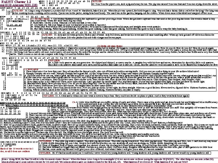
FAUST Cluster 1. 2 WS 0= 2 3 13 20 22 25 38 42 44 49 50 OUTLIER: DS 1= | WS 1= 2 20 25 46 49 51 46. Tom the piper's son, stole a pig and away he run. The pig was eat and Tom was beat and Tom ran crying down the street. 46 | DS 2 46 DS 0=|WS 1= 7 10 17 23 25 28 33 34 37 40 43 45 50 35 |---|OUTLIER: 35. Sing a song of sixpence, a pocket full of rye. 4 and 20 blackbirds, baked in a pie. When the pie was opened, the birds began to sing. Was not that a dainty dish to set before the king? The king was |DS 2| |35 |in his counting house, counting out his money. Queen was in the parlor, eating bread and honey. The maid was in the garden, hanging out the clothes. When down came a blackbird and snapped off her nose. WS 0= 2 3 13 32 38 42 44 52 DS 1 |WS 1= 42(Mother) C 1: Mother theme 7. Old Mother Hubbard went to the cupboard to give her poor dog a bone. When she got there cupboard was bare and so the poor dog had none. She went to baker to buy him some bread. When she came back dog was dead. 7 9 |DS 2|WS 2=WS 1 9. Hush baby. Daddy is near. Mamma is a lady and that is very clear. 11 |7 27. Cry baby cry. Put your finger in your eye and tell your mother it was not I. 27 |9 27 29 45 29. When little Fred went to bed, he always said his prayers. He kissed his mamma and then his papa, and straight away went upstairs. 29 45. Bye baby bunting. Father has gone hunting. Mother has gone milking. Sister has gone silking. And brother has gone to buy a skin to wrap the baby bunting in. 32 29 41 45 DS 0|WS 1 2 9 12 18 19 21 26 27 30 32 38 39 42 44 45 47 49 52 54 55 57 60 1 |DS 1| WS 2 12 19 26 39 44 OUTLIER: 10. Jack and Jill went up hill to fetch a pail of water. Jack fell down, and broke his crown and Jill came tumbling after. When up Jack got and off did trot as fast as he 10 | DS 2| WS 3 could caper, to old Dame Dob who patched his nob with vinegar and brown paper. 13 | | 10 | DS 3 10 17 37 14 39 21 41 26 44 28 30 47 50 WS 0 22 38 44 52 DS 1 WS 1= 27 38 44 {fiddle(32 41) man(11 32) old(11 44) C 2 fiddle old man theme 11 DS 211. One misty morning when cloudy was weather, I chanced to meet an old man clothed all in leather. He began to compliment and I began to grin. How do you do? How do you do again 32 11 32. Jack come and give me your fiddle, if ever you mean to thrive. No I will not give my fiddle to any man alive. If I'd give my fiddle they will think I've gone mad. For many a joyous day my fiddle and I have had 41 22 41. Old King Cole was a merry old soul. And a merry old soul was he. He called for his pipe and he called for his bowl and he called for his fiddlers three. And every fiddler, he had a fine fiddle and a very fine fiddle 44 had he. There is none so rare as can compare with King Cole and his fiddlers three. real HOB Alternate WS 0, DS 0| WS 1=2 9 18 21 30 38 41 45 47 49 52 54 55 57 60 1 | DS 1|WS 2=2 9 18 30 39 45 55 OUTLIER: 13 | 39 |DS 2 39. A little cock sparrow sat on a green tree. He chirped and chirped, so merry was he. A naughty boy with his bow and arrow, determined to shoot this little cock sparrow. 14 | |39 This little cock sparrow shall make me a stew, and his giblets shall make me a little pie. Oh no, says the sparrow I will not make a stew. So he flapped his wings, away he flew 17 21 39 28 41 30 47 37 50 C 3: men three 1. Three blind mice! See how they run! They all ran after the farmer's wife, who cut off their tails with a carving knife. Did you ever see such a thing in your life as three blind mice? WS 0 38 52 5. Humpty Dumpty sat on a wall. Humpty Dumpty had a great fall. All the Kings horses, and all the Kings men cannot put Humpty Dumpty together again. DS 1 WS 1= 38 52 14. If all the seas were one sea, what a great sea that would be! And if all the trees were one tree, what a great tree that would be! And if all the axes were one axe, what a great axe that would be! And 1 ----- if all the men were one man what a great man he would be! And if the great man took the great axe and cut down the great tree and let it fall into the great sea, what a splish splash that would be! 5 17. Here sits the Lord Mayor. Here sit his two men. Here sits the cock. Here sits the hen. Here sit the little chickens. Here they run in. Chin chopper, chin! 17 23. How many miles is it to Babylon? Three score miles and ten. Can I get there by candle light? Yes, and back again. If your heels are nimble and light, you may get there by candle light. 23 28. Baa black sheep, have you any wool? Yes sir yes sir, three bags full. One for my master and one for my dame, but none for the little boy who cries in the lane. 28 36. Little Tommy Tittlemouse lived in a little house. He caught fishes in other mens ditches. 36 48. One two, buckle my shoe. Three four, knock at the door. Five six, pick up sticks. Seven eight, lay them straight. Nine ten. a good fat hen. Eleven twelve, dig and delve. Thirteen fourteen, maids a 48 courting. Fifteen sixteen, maids in the kitchen. Seventeen eighteen. maids a waiting. Nineteen twenty, my plate is empty. DS 0|WS 1 2 5 8 13 14 15 16 22 24 25 29 36 41 44 47 48 51 54 57 59 13 |DS 2|WS 2 4 13 47 51 54 OUTLIER: 13. A robin and a robins son once went to town to buy a bun. They could not decide on plum or plain. And so they went back home again. 14 |13 |DS 3 13 21 26 30 37 47 50 C 4: 4. Little Miss Muffet sat on a tuffet, eating of curds and whey. There came a big spider and sat down beside her and frightened Miss Muffet away. WS 0=2 5 8 11 14 15 16 22 24 25 29 31 36 41 44 47 48 53 54 57 59 6. See a pin and pick it up. All the day you will have good luck. See a pin and let it lay. Bad luck you will have all the day. DS 1|WS 1(17 wds)=2 5 11 15 16 22 24 25 29 31 41 44 47 48 54 57 59 8. Jack Sprat could eat no fat. Wife could eat no lean. Between them both they licked platter clean. 4 6 8|DS 2=DS 1 12. There came an old woman from France who taught grown-up children to dance. But they were so stiff she sent them home in a sniff. This sprightly old woman from France. 12 15 18 21 15. Great A. little a. This is pancake day. Toss the ball high. Throw the ball low. Those that come after may sing heigh ho! 18. I had two pigeons bright and gay. They flew from me the other day. What was the reason they did go? I can not tell, for I do not k 25 26 30 33 37 21. Lion and Unicorn were fighting for crown. Lion beat Unicorn all around town. Some gave them white bread and some gave them brown. Some gave them plum cake, and sent them out of town. 43 44 47 49 50 25. There was an old woman, and what do you think? She lived upon nothing but victuals, and drink. Victuals and drink were the chief of her diet, and yet this old woman could never be quiet. 26. Sleep baby sleep. Our cottage valley is deep. Little lamb is on green with woolly fleece so soft, clean. Sleep baby sleep, down where woodbines creep. Be always like lamb so mild, a kind and sweet and gentle child. Sleep baby sleep. 30. Hey diddle! The cat and the fiddle. The cow jumped over the moon. The little dog laughed to see such sport, and the dish ran away with the spoon. 33. Buttons, a farthing a pair! Come, who will buy them of me? They are round and sound and pretty and fit for girls of the city. Come, who will buy them of me? Buttons, a farthing a pair! 37. Here we go round mulberry bush, mulberry bush. Here we go round mulberry bush, on a cold and frosty morning. This is way we wash our hands, wash our hands. This is way we wash our hands, on a cold and frosty morning. This is way we wash our clothes, wash our clothes. This is way we wash our clothes, on a cold and frosty morning. This is way we go to school, go to school. This is the way we go to school, on a cold and frosty morning. This is the way we come out of school, come out of school. This is the way we come out of school, on a cold and frosty morning. 43. Hark hark, the dogs do bark! Beggars are coming to town. Some in jags and some in rags and some in velvet gowns. 44. The hart he loves the high wood. The hare she loves the hill. The Knight he loves his bright sword. The Lady loves her will. 47. Cocks crow in the morn to tell us to rise and he who lies late will never be wise. For early to bed and early to rise, is the way to be healthy and wise. 49. There was a little girl who had a little curl right in the middle of her forehead. When she was good she was very good and when she was bad she was horrid. 50. Little Jack Horner sat in the corner, eating of Christmas pie. He put in his thumb and pulled out a plum and said What a good boy am I! DS 0|WS 1=6 7 8 14 43 46 48 51 53 57 OUTLIERS: 2. This little pig went to market. This little pig stayed home. This little pig had roast beef. This little pig had none. This little pig said Wee, wee. I can't find my way home 3. Diddle dumpling, my son John. Went to bed with his breeches on, one stocking off, and one stocking on. Diddle dumpling, my son John. 2 3|DS 2=DS 1 16. Flour of England, fruit of Spain, met together in a shower of rain. Put in a bag tied round with a string. If you'll tell me this riddle, I will give you a ring. 16 22 42 22. Had little husband no bigger than my thumb. Put him in a pint pot, there I bid him drum. Bought a little handkerchief to wipe his little nose, pair of little garters to tie little hose Each of the 10 words occur in 1 42. Bat bat, come under my hat and I will give you a slice of bacon. And when I bake I will give you a cake, if I am not mistaken. doc, so all 5 docs are outliers OUTLIER: 38. If I had as much money as I could tell, I never would cry young lambs to sell. Young lambs to sell, young lambs to sell. I never would cry young lambs to sell. Notes Using HOB, the final Word. Set is the document cluster theme! When theme is too long to be meaningful (C 4) we can recurse on those (using the opposite DS)|WS 0? ). The other thing we can note is that DS) almost always gave us an outliers (except for C 5) and only WS) almost always gave us clusters (excpt for the first one, 46). What happens if we reverse it? What happens if we just use WS 0?
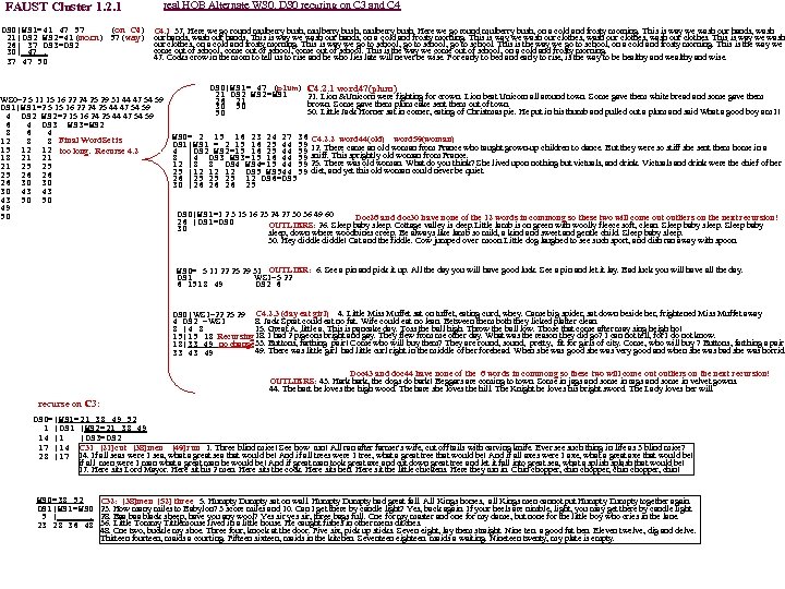
FAUST Cluster 1. 2. 1 DS 0|WS 1=41 47 57 (on C 4) 21|DS 2 WS 2=41(morn) 57(way) 26| 37 DS 3=DS 2 30| 47. 37 47 50 real HOB Alternate WS 0, DS 0 recuring on C 3 and C 4. 1 37. Here we go round mulberry bush, mulberry bush. Here we go round mulberry bush, on a cold and frosty morning. This is way we wash our hands, wash our hands. This is way we wash our hands, on a cold and frosty morning. This is way we wash our clothes, wash our clothes. This is way we wash our clothes, on a cold and frosty morning. This is way we go to school, go to school. This is the way we go to school, on a cold and frosty morning. This is the way we come out of school, come out of school. This is the way we come out of school, on a cold and frosty morning. 47. Cocks crow in the morn to tell us to rise and he who lies late will never be wise. For early to bed and early to rise, is the way to be healthy and wise. WS 0=2 5 11 15 16 22 24 25 29 31 44 47 54 59 DS 1|WS 1=2 5 15 16 22 24 25 44 47 54 59 4 DS 2 WS 2=2 15 16 24 25 44 47 54 59 6 4 DS 3 WS 3=WS 2 8 6 4 12 8 8 Final Word. Set is 15 12 12 too long. Recurse 4. 2 18 21 21 21 25 25 25 26 26 26 30 30 30 43 43 43 50 50 49 50 DS 0|WS 1= 47 (plum) 21 DS 2 WS 2=WS 1 26 21 30 50 50 C 4. 2. 1 word 47(plum) 21. Lion &Unicorn were fighting for crown. Lion beat Unicorn all around town. Some gave them white bread and some gave them brown. Some gave them plum cake sent them out of town. 50. Little Jack Horner sat in corner, eating of Christmas pie. He put in his thumb and pulled out a plum and said What a good boy am I! WS 0= 2 15 16 23 24 27 36 DS 1|WS 1 = 2 15 16 25 44 59 4 |DS 2 WS 2=15 16 25 44 59 8 |4 DS 3 WS 3=15 16 44 59 12 |8 8 DS 4 WS 4=15 44 59 25 |12 12 12 DS 5 WS 544 59 26 |25 25 25 12 DS 6=DS 5 30 |26 26 26 25 C 4. 2. 2 word 44(old) word 59(woman) 12. There came an old woman from France who taught grown-up children to dance. But they were so stiff she sent them home in a sniff. This sprightly old woman from France. 25. There was old woman. What do you think? She lived upon nothing but victuals, and drink. Victuals and drink were the chief of her diet, and yet this old woman could never be quiet. DS 0|WS 1=1 2 3 15 16 23 24 27 30 36 49 60 Doc 26 and doc 30 have none of the 12 words in commong so these two will come outliers on the next recursion! 26 |DS 1=DS 0 OUTLIERS: 26. Sleep baby sleep. Cottage valley is deep. Little lamb is on green with woolly fleece soft, clean. Sleep baby sleep. Sleep baby 30 sleep, down where woodbines creep. Be always like lamb so mild, a kind and sweet and gentle child. Sleep baby sleep. 30. Hey diddle! Cat and the fiddle. Cow jumped over moon. Little dog laughed to see such sport, and dish ran away with spoon. WS 0= 5 11 22 25 29 31 OUTLIER: 6. See a pin and pick it up. All the day you will have good luck. See a pin and let it lay. Bad luck you will have all the day. DS 1 WS 1=5 22 6 1518 49 DS 2 6 DS 0|WS 1=22 25 29 C 4. 2. 3 (day eat girl) 4. Little Miss Muffet sat on tuffet, eating curd, whey. Came big spider, sat down beside her, frightened Miss Muffet away 8. Jack Sprat could eat no fat. Wife could eat no lean. Between them both they licked platter clean. 4 DS 2 =WS 1 15. Great A. little a. This is pancake day. Toss the ball high. Throw the ball low. Those that come after may sing heigh ho! 8 |4 8 15|15 18 Recursing 18. I had 2 pigeons bright and gay. They flew from me other day. What was the reason they did go? I can not tell, for I do not know. 18|33 49 no change 33. Buttons, farthing pair! Come who will buy them? They are round, sound, pretty, fit for girls of city. Come, who will buy ? Buttons, farthing a pair 49. There was little girl had little curl right in the middle of her forehead. When she was good she was very good and when she was bad she was horrid. 33 43 49 Doc 43 and doc 44 have none of the 6 words in commong so these two will come outliers on the next recursion! OUTLIERS: 43. Hark hark, the dogs do bark! Beggars are coming to town. Some in jags and some in rags and some in velvet gowns. 44. The hart he loves the high wood. The hare she loves the hill. The Knight he loves his bright sword. The Lady loves her will. recurse on C 3: DS 0=|WS 1=21 38 49 52 1 |DS 1 |WS 2=21 38 49 14 |1 |DS 3=DS 2 17 |14 C 31 [21]cut [38]men [49]run 1. Three blind mice! See how run! All ran after farmer's wife, cut off tails with carving knife. Ever see such thing in life as 3 blind mice? 28 |17 14. If all seas were 1 sea, what a great sea that would be! And if all trees were 1 tree, what a great tree that would be! And if all axes were 1 axe, what a great axe that would be! if all men were 1 man what a great man he would be! And if great man took great axe and cut down great tree and let it fall into great sea, what a splish splash that would be! 17. Here sits Lord Mayor. Here sit his 2 men. Here sits the cock. Here sits hen. Here sit the little chickens. Here they run in. Chin chopper, chin! WS 0=38 52 DS 1|WS 1=WS 0 5 |. 23 28 36 48 C 32: [38]men [52] three 5. Humpty Dumpty sat on wall. Humpty Dumpty had great fall. All Kings horses, all Kings men cannot put Humpty Dumpty together again. 23. How many miles to Babylon? 3 score miles and 10. Can I get there by candle light? Yes, back again. If your heels are nimble, light, you may get there by candle light. 28. Baa black sheep, have you any wool? Yes sir yes sir, three bags full. One for my master and one for my dame, but none for the little boy who cries in the lane. 36. Little Tommy Tittlemouse lived in a little house. He caught fishes in other mens ditches. 48. One two, buckle my shoe. Three four, knock at the door. Five six, pick up sticks. Seven eight, lay them straight. Nine ten. a good fat hen. Eleven twelve, dig and delve. Thirteen fourteen, maids a courting. Fifteen sixteen, maids in the kitchen. Seventeen eighteen. maids a waiting. Nineteen twenty, my plate is empty.
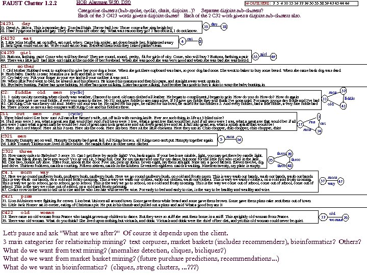
FAUST Cluster 1. 2. 2 HOB Alternate WS 0, DS 0 16 OUTLIERS: 2 3 6 10 13 16 22 26 30 35 38 39 42 43 44 46 Categorize clusters (hub-spoke, cyclic, chain, disjoint. . . )? Separate disjoint sub-clusters? Each of the 3 C 423 words gives a disjoint cluster! Each of the 2 C 32 work gives a disjoint sub-clusters also. C 4231 day C 4232 eat C 4233 girl 15 15. Great A. little a. This is pancake day. Toss ball high. Throw ball low. Those come after sing heigh ho! 18. I had 2 pigeons bright and gay. They flew from me other day. What was reason they go? I can not tell, I do not know. 4. Little Miss Muffet sat on tuffet, eat curd, whey. Came big spider, sat down beside her, frightened away 8. Jack Sprat could eat no fat. Wife could eat no lean. Between them both they licked platter clean. 4 eat day 18 8 33. Buttons, farthing pair! Come who will buy them? They are round, sound, pretty, fit for girls of city. Come, who will buy ? Buttons, farthing a pair 49. There was little girl had little curl right in the middle of her forehead. When she was good she was very good and when she was bad she was horrid. C 1: 33 girl 49 mother 7. Old Mother Hubbard went to cupboard to give her poor dog a bone. When she got there cupboard was bare, so poor dog had none. She went to baker to buy some bread. When she came back dog was dead. 9. Hush baby. Daddy is near. Mamma is a lady and that is very clear. 27. Cry baby cry. Put your finger in your eye and tell your mother it was not I. 29. When little Fred went to bed, he always said his prayers. He kissed his mamma and then his papa, and straight away went upstairs. 45. Bye baby bunting. Father has gone hunting. Mother has gone milking. Sister has gone silking. And brother has gone to buy a skin to wrap the baby bunting in. C 2: fiddle old men {cyclic} 11. 1 misty morning when cloudy was weather, Chanced to meet old man clothed all leather. He began to compliment, I began to grin. How do you do How do? How do again 32. Jack come give me your fiddle, if ever you mean to thrive. No I'll not give fiddle to any man alive. If I'd give my fiddle they will think I've gone mad. For many joyous day fiddle and I've had 11 41. Old King Cole was merry old soul. Merry old soul was he. He called for his pipe, he called for his bowl, he called for his fiddlers 3. And every fiddler, had a fine fiddle, a very fine fiddle had old he. There is none so rare as can compare with King Cole and his fiddlers three. C 11 cut C 321 men C 322 men run 32 fiddle 41 {cyclic} three 1 1. Three blind mice! See how run! All ran after farmer's wife, cut off tails with carving knife. Ever see such thing in life as 3 blind mice? 14. If all seas were 1 sea, what a great sea that would be! And if all trees were 1 tree, what a great tree that would be! And if all axes were 1 axe, what a great axe that would be! if all run cut 17 men were 1 man what a great man he would be! And if great man took great axe and cut down great tree and let it fall into great sea, what a splish splash that would be! 17. Here sits Lord Mayor. Here sit his 2 men. Here sits the cock. Here sits hen. Here sit the little chickens. Here they run in. Chin chopper, chin! men 14 5. Humpty Dumpty sat on wall. Humpty Dumpty had great fall. All Kings horses, all Kings men can't put Humpty together again. 36. Little Tommy Tittlemouse lived in little house. He caught fishes in other mens ditches. 5 men 36 23. How many miles to Babylon? 3 score 10. Can I get there by candle light? Yes, back again. If your heels are nimble, light, you may get there by candle light. 28. Baa black sheep, have any wool? Yes sir yes sir, 3 bags full. One for my master and one for my dame, but none for the little boy who cries in the lane. 48. One two, buckle my shoe. Three four, knock at the door. Five six, pick up sticks. Seven eight, lay them straight. Nine ten. a good fat hen. Eleven twelve, dig and delve. Thirteen fourteen, maids a courting. Fifteen sixteen, maids in the kitchen. Seventeen eighteen. maids a waiting. Nineteen twenty, my plate is empty. C 4. 1 morn 23 three 28 three 48 way 37. Here we go round mulberry bush, mulberry bush. Here we go round mulberry bush, on cold and frosty morn. This is way wash our hands, wash our hands. This is way wash our hands, on a cold and frosty morning. This is way we wash our clothes, wash our clothes. This is way we wash r clothes, on a cold and frosty morning. This is way we go to school, go to school. This is the way we go to school, on a cold and frosty morning. This is the way we come out of school, come out of school. This is the way we come out of school, on a cold and frosty morning. 47. Cocks crow in the morn to tell us to rise and he who lies late will never be wise. For early to bed and early to rise, is the way to be healthy and wise. C 421 old morn way 47 plum C 422 37 21. Lion &Unicorn were fighting for crown. Lion beat Unicorn all around town. Some gave them white bread and some gave them brown. Some gave them plum cake sent them out of town. 50. Little Jack Horner sat in corner, eating of Christmas pie. He put in his thumb and pulled out a plum and said What a good boy am I! woman 12. There came an old woman from France who taught grown-up children to dance. But they were so stiff she sent them home in a sniff. This sprightly old woman from France. 25. There was old woman. What do you think? She lived upon nothing but victuals, and drink. Victuals and drink were the chief of her diet, and yet this old woman could never be quiet. 12 old woman 25 Let's pause and ask "What are we after? " Of course it depends upon the client. 3 main categories for relatioinship mining? text corpuses, market baskets (includes recommenders), bioinformatics? Others? What do we want from text mining? (anomalies detection, cliques, bicliques? ) What do we want from market basket mining? (future purchase predictions, recommendations. . . ) What do we want in bioinformatics? (cliques, strong clusters, . . . ? ? ? )
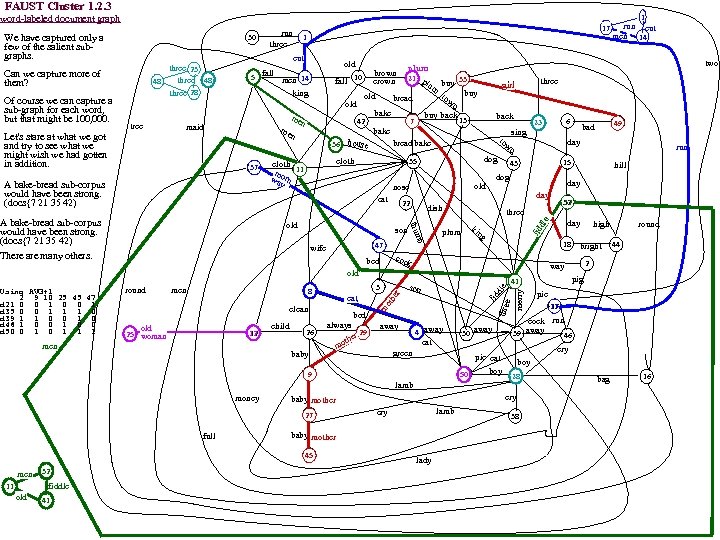
FAUST Cluster 1. 2. 3 word-labeled document graph 1 30 Let's stare at what we got and try to see what we might wish we had gotten in addition. 1 cut three 23 three 48 48 three 28 Can we capture more of them? Of course we can capture a sub-graph for each word, but that might be 100, 000. run three old 5 fall men 14 fall 10 king old tree me n maid 37 A bake-bread sub-corpus would have been strong. (docs{7 21 35 42) bake 42 36 house cloth back 13 to thum son ki ng k old 25 woman 12 men child 26 baby eat bed always 29 er oth m away dle e merry clean 4 away eat green pie eat boy 50 50 9 lamb money full baby mother 45 men 32 old 41 fiddle 11 lamb cry lady pie 17 cock run away 39 46 cry boy 28 cry baby mother 27 30 away 44 pig 41 41 son fid 3 8 thre men mo the r round 2 way old Using AVG+1 2 9 10 25 45 47 d 21 0 0 1 d 35 0 0 1 1 1 0 d 39 1 1 0 0 1 0 d 46 1 0 0 d 50 0 1 1 1 high 18 bright coc bed day b 47 wife 32 three plum hill day dish run 15 43 dog old nose 49 bad day wn 35 old 6 23 sing dog 22 three girl bread bake eat A bake-bread sub-corpus would have been strong. (docs{7 21 35 42) There are many others. buy back 7 bake cloth 11 m wa orn y 33 m buy to buy wn bread run cut men 14 two plum 21 p lu brown crown fid dle We have captured only a few of the salient subgraphs. 17 38 bag 16
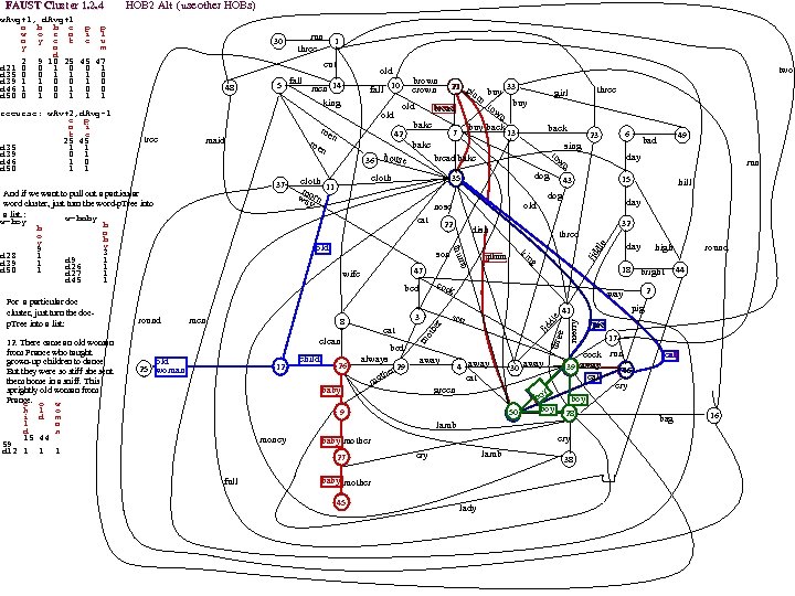
HOB 2 Alt (use other HOBs) fall 10 old 36 house 22 son 47 wife 12 child 26 baby bed always 29 er oth m ng away 4 away eat 30 green 50 50 away e pey pii oy bo boy 27 full baby mother 45 lady 17 cock run eat 46 46 cry boy 28 cry lamb cry 44 pie 39 away lamb baby mother round pig 41 son high 2 way 9 money day 18 bright k 3 eat ki thre clean 32 three plum hill day coc bed 8 dish run 15 43 dog old nose old 25 woman dog 49 bad day wn 35 35 eat 6 23 sing to bread bake cloth 11 m wa orn y men back 13 bake n 37 buy back 7 dle me bake 42 n bread three girl b round me 33 m buy to buy wn 21 p 21 l u fid maid old r tree brown crown dle e merry 48 two old fall 5 men 14 king thum 12. There came an old woman from France who taught grown-up children to dance. But they were so stiff she sent them home in a sniff. This sprightly old woman from France. o w c h l o i d m l a d n 15 44 59 d 12 1 1 cut And if we want to pull out a particular word cluster, just turn the word-p. Tree into a list. : w=baby w=boy a b w a w o b a y 2 9 2 3 d 28 0 1 d 9 0 1 d 39 1 1 d 26 1 1 d 50 0 1 d 27 0 1 d 45 1 For a particular doc cluster, just turn the docp. Tree into a list: run three the recurse: w. Av+2, d. Avg-1 e p a i t e 2 9 10 25 45 d 35 0 0 1 1 1 d 39 1 1 0 0 1 d 46 1 0 0 1 0 d 50 0 1 1 30 fid w. Avg+1, d. Avg+1 a b b e p p w o r a i l a y e t e u y a m d 2 9 10 25 45 47 d 21 0 0 1 d 35 0 0 1 1 1 0 d 39 1 1 0 0 1 0 d 46 1 0 0 d 50 0 1 1 1 mo FAUST Cluster 1. 2. 4 38 bag 16
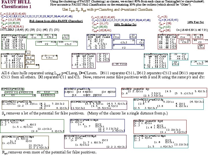
FAUST HULL Classification 1 Using the clustering of FAUST Clustering 1 as classes, we extract 80% from each class as Training. Set (w class=cluster#). How accurate is FAUST Hull Classification on the remaining 20% plus the outliers (which should be "Other"). Use Lpd, Sp, Rpd with p=Class. Avg and d=unitized Class. Sum. C 11={2, 3, 16, 22, 43} C 2 ={1, 4, 5, 8, 9, 12, 14, 15, 23, 25, 27, 32, 33, 36, 37, 38, 44, 45, 47, 48} C 311= {11, 17, 29} Full classes from slide: FAUST Clustering 1 C 312={13, 30, 50} C 313={10, 26, 28, 41} OUTLIERS {18, 49} {6} {39} {21} {46} {7} {35} C 11={2, 16, 22, 43} C 2 ={1, 5, 8, 9, 12, 15, 27, 32, 33, 36, 37, 38, 44, 47, 48} C 311= {11, 17} 80% Training Set C 312={30, 50} C 313={10, 28, 41} D 11= C 11 p=av. C 11 L 0 D 1= TS p=av. TS Lpd -. 09. 106. 305. 439. 572 C 312 MIN MAX CLASS C 311 C 11 MIN MAX CLASS C 311. 63 C 11 -0. 09. 106 C 11 0 0. 63 C 2 0. 106. 439 C 2. 106. 439. 505. 771 C 313 0 0 C 311 0. 572 C 311 C 2 C 313 0. 31 C 312 0. 305. 439 C 312 C 2 0. 31 C 313 0. 505. 771 C 313 0 D 312= C 312 p=av. C 312. 31 C 11 D 311= C 311 p=av. C 311 C 11 1. 3 1. 6 L MN MX CLAS. 31 C 2 L MN MX CLAS 0. 33 C 311 C 312 0. 31 C 11. 31 C 311 0 0 C 11 0. 31 C 2. 31 C 313 0 0. 66 C 2 0. 33 0. 31 C 311 1. 33 1. 66 C 311 C 313 1. 58 C 312 0 0. 33 C 312 0. 66 0. 31 C 313 0 0. 33 C 313 C 2 . 31 C 312. 31 C 11={3} C 2 ={4, 14, 23, 45} 20% Test Set C 311= {29} C 312={13} O={18 49 6 39 21 46 7 35} C 313={26} D 2= C 2 p=av. C 2 L 0 MIN 0. 44. 66. 11. 44 . 63 C 11. 63 . 22. 44. 66 MAX CLS C 11 C 313. 22 C 11. 22. 44. 77 C 2 C 312 C 2. 66 C 311. 66. 22 C 311. 66 C 313 D 313= C 313 p=av. C 313 0. 22 L MN MX 0. 22 0. 44 0. 22 1. 34 1. 56 CLAS C 11 C 2 C 311 C 312 C 313 0 0 C 11. 44 C 2. 44 C 311 1. 34 1. 56. 22 C 313 C 312 All 6 class hulls separated using Lpd, p=CLavg, D=CLsum. D 311 separates C 311, D 312 separates C 312 and D 313 separates C 313 from all others. D 2 separates C 11 and C 2. Now, remove some false positives with S and R using the same p's and d's: D 1= TS p=av. TS Sp 4. 2 C 313 5. 4 1. 9 C 11 2. 4 C 311 3. 4 4. 6 C 312 4. 7 1. 8 C 2 3. 8 D 11= C 11 p=av. C 11 Sp [1. 6]C 11 [3. 4 4 4]C 311 [5. 4 6]C 313 [2. 4 4. 4]C 2 [5]C 312 D 2= C 2 p=av. C 2 Sp [1. 8 D 311= C 311 p=av. C 311 Sp D 312= C 312 p=av. C 312 Sp [1. 2]C 311 [4. 2]C 11 [6. 2 7. 2]C 312 [3. 5 4. 5]C 11 [6. 5 7. 5]C 313 [2. 2 6. 2]C 2 [4. 5 6. 5]C 2 [6. 2 8. 2]C 313 [2. 5]C 312 [5. 5]C 311 [2 2. 3]C 11 3. 5]C 2 [2. 5 3. 5]C 311 [4. 5 [5 5. 1]C 312 D 313= C 313 p=av. C 313 Sp [3. 5 4. 2]C 11 [6. 5]C 312 [2. 8 6. 2]C 2 [3. 8 6. 2]C 311 [2. 5 3. 5]C 313 Sp removes a lot of the potential for false positives. (Many of the classes lie a single distance from p. ) D 1= TS p=av. TS Rpd [1. 3 1. 4]C 11 [1. 3 1. 9]C 2 [1. 5 1. 8]C 311 [2. 1]C 312 [2. 0 D 311= C 311 p=av. C 311 Rpd [1. 4]C 11 [1. 2 2]C 2 [1. 1]C 311 [2. 2]C 312 [2. 2 2. 4]C 313 2. 2]C 313 D 11= C 11 p=av. C 11 Rpd [1. 2]C 11 [1. 4 2]C 2 [1. 7 2]C 311 [2. 2 2. ]]C 312 [2. 2 2. 4]C 313 D 312= C 312 p=av. C 312 Rpd [1. 3 1. 4]C 11 [1. 4 2]C 2 [1. 7 1. 9]C 311 [1. 5]C 312 [2. 2 2. 4]C 313 Rpd removes even more of the potential for false positives. 5. 8]C 313 D 2= C 2 p=av. C 2 Rpd [1. 3 1. 4]C 11 [1. 3 1. 8]C 2 [1. 6 1. 8]C 311 [2. 2]C 312 2. 4]C 313 D 313= C 313 p=av. C 313 Rpd [1. 3 1. 4]C 11 [1. 3 2]C 2 [1. 6 2]C 311 [1. 5 1. 8]C 313 [2. 2]C 312
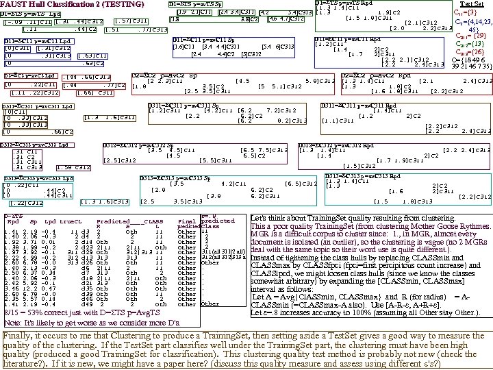
D 1= TS p=av. TS Rpd D 1= TS p=av. TS Sp Test Set [1. 3 1. 4]C 11 [1. 9 2. 1]C 11 [2. 4 3. 4]C 311 [4. 2 5. 4]C 313 [1. 3 C 11={3} 1. 9]C 2 D 1= TS p=av. TS Lpd [1. 5 1. 8]C 311 [4. 6 4. 7]C 312 [1. 8 3. 8]C 2 [. 57]C 311 C 2 ={4, 14, 23, [-. 09. 11]C 11 [. 31. 44]C 312 [2. 1]C 312 [2. 0 2. 2]C 313 45} [. 11. 44]C 2 [. 51. 77]C 313 FAUST Hull Classification 2 (TESTING) D 11= C 11 p=av. C 11 Lpd [0]C 311 [. 31]C 312 [0. 31]C 313 [0 [. 63]C 11. 63]C 2 D 2= C 2 p=av. C 2 Lpd . [44. 66]C 313 [0. 22]C 11 [. 44. 77]C 2 [. 66] C 311 [. 11. 22]C 312 D 2= C 2 p=av. C 2 Sp [1. 3 D 312= C 312 p=av. C 312 Lpd . 31. 31 C 11 C 2 C 311 C 313 1. 58 C 312 1. 6]C 311 D= TS Rpd 1. 41 1. 40 1. 92 1. 38 1. 97 2. 22 2. 60 1. 40 2. 50 1. 40 2. 42 3. 46 2. 60 2. 35 1. 41 Sp 2. 19 2. 06 3. 71 1. 99 3. 92 4. 99 6. 78 2. 13 6. 37 2. 06 5. 92 12. 2 6. 78 5. 57 2. 19 [1. 3 1. 6]C 313 Lpd true. CL -0. 4 -0. 3 0. 01 -0. 2 -0. 0 -0. 34 -0. 3 -0. 1 0. 47 -0. 0 0. 14 -0. 4 11 2 2 2 311 312 313 d 4 d 14 d 23 d 29 d 13 d 26 d 7 d 18 d 21 d 35 d 39 d 46 d 49 3. 5]C 2 [2. 5 3. 5]C 311 [4. 5 [5 5. 1]C 312 5. 8]C 313 D 311= C 311 p=av. C 311 Sp [1. 2]C 311 [4. 2]C 11 [6. 2 7. 2]C 312 [2. 2 6. 2]C 2 [6. 2 8. 2]C 313 D 312= C 312 p=av. C 312 Sp [3. 5 4. 5]C 11 [4. 5 [2. 5]C 312 [5. 5]C 311 D 313= C 313 p=av. C 313 Lpd [0. 22]C 11 [0. 44]C 2 [0. 44]C 311 [. 22]C 312 [2 2. 3]C 11 [1. 8 D 311= C 311 p=av. C 311 Lpd [0]C 11 [0. 33]C 312 [0. 33]C 313 [0. 66]C 2 D 11= C 11 p=av. C 11 Rpd [1. 2]C 11 [1. 4 2]C 2 [1. 7 2]C 311 [2. 2 2. ]]C 312 [2. 2 2. 4]C 313 D 11= C 11 p=av. C 11 Sp [1. 6]C 11 [3. 4 4 4]C 311 [5. 4 6]C 313 [2. 4 4. 4]C 2 [5]C 312 [6. 5 7. 5]C 313 6. 5]C 2 Predicted____CLASS R S L 2 Oth 11 2 2 11 Oth 2 11 2|11 Oth 312|313 11 Oth 11 2|11 2 11 313 Oth 2 2|11 Oth 313 Oth Oth 11 Oth 2 2 2 Oth ε=. 8 Final predicted Class Other 11 Other 2 Other 311(all 311|2 all) Other 312(all 312|313 a Other. Other 8/15 = 53% correct just with D= TS p=Avg. TS Note: It's likely to get worse as we consider more D's. D 2= C 2 p=av. C 2 Rpd [1. 3 1. 4]C 11 [2. 1 2. 4]C 313 [1. 3 1. 8]C 2 [1. 6 1. 8]C 311 [2. 2]C 312 D 311= C 311 p=av. C 311 Rpd [1. 4]C 11 [1. 2 2]C 2 [1. 1]C 311 D 312= C 312 p=av. C 312 Rpd [1. 3 1. 4]C 11 [1. 4 [1. 5]C 312 D 313= C 313 p=av. C 313 Sp [3. 5 4. 2]C 11 [6. 5]C 312 [2. 8 6. 2]C 2 [3. 8 6. 2]C 311 [2. 5 3. 5]C 313 C 311= {29} C 312={13} C 313={26} O={18 49 6 39 21 46 7 35} [1. 7 1. 9]C 311 [2. 2]C 312 [2. 2 2. 4]C 313 2]C 2 D 313= C 313 p=av. C 313 Rpd [1. 3 1. 4]C 11 [1. 3 [1. 6 [1. 5 [2. 2 2. 4]C 313 2]C 2 2]C 311 1. 8]C 313 [2. 2]C 312 Let's think about Training. Set quality resulting from clustering. This a poor quality Training. Set (from clustering Mother Goose Rythmes. MGR is a difficult corpus to cluster since: 1. , in MGR, almost every document is isolated (an outlier), so the clustering is vague (no 2 MGRs deal with the same topic so their word use is quite different. ). Instead of tightening the class hulls by replacing CLASSmin and CLASSmax by CLASSfpci (fpci=first percipitous count increase) and CLASSlpcd, we might loosen class hulls (since we know the classes somewhat arbitrary) by expanding the [CLASSmin, CLASSmax] interval as follows: Let A = Avg{Cl. ASSmin, CLASSmax} and R (for radius) = ACLASSmin (=CLASSmax-A also). Use [A-R-ε, A+R+ε]. Let ε=. 8 increases accuracy to 100% (assuming all Other stay Other. ). Finally, it occurs to me that Clustering to produce a Training. Set, then setting aside a Test. Set gives a good way to measure the quality of the clustering. If the Test. Set part classifies well under the Training. Set part, the clustering must have been high quality (produced a good Training. Set for classification). This clustering quality test method is probably not new (check the literature? ). If it is new, we might have a paper here? (discuss this quality measure and assess using different ε's? )
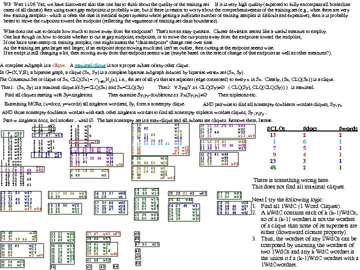
WP Wed 11/26 Yes, we have discovered also that one has to think about the quality of the training set. If it is very high quality (expected to fully encompass all borderline cases of all classes) then using exact gap endpoints is probably wise, but if there is reason to worry about the comprehensiveness of the training set (e. g. , when there are very few training samples - which is often the case in medical expert systems where getting a sufficient number of training samples is difficult and expensive), then it is probably better to move the cutpoints toward the midpoint (reflecting the vagueness of training set class boundaries). What does one use to decide how much to move away from the endpoints? That's not an easy question. Cluster deviation seems like a useful measure to employ. One last though on how to decide whether to cut at gap midpoint, endpoints, or to move the cut-points away from the endpoints toward the midpoint, If one has a time-stamp on training samples, one might assess the "class endpoint" change rate over time. As the training set gets larger and larger, if an endpoint stops moving much and isn't an outlier, then cutting at the endpoint seems wise. If an endpt is still changing a lot, then moving away from that endpoint seems wise (maybe based on the rate of change of that endpoint as well as other measures? ). A complete subgraph is a clique. A maximal clique is not a proper subset of any other clique. In G=(X, Y, E), a bipartite graph, a clique (Sx, Sy) is a complete bipartite subgraph induced by bipartite vertex set (Sx, Sy). The Consensus Set or clique of Sx, CLQ(Sx) = x Sx. Ny(x), i. e. , the set of all y's that are adjacent (edge connected) to every x in Sx. Clearly, (Sx, CLQ(Sx)) is a clique. Thm 2: Sy Y s. t. CLQ(Sy) ( CLQ(Sy), CLQ(Sy)) ) is maximal. Thm 1: (Sx, Sy) is a maximal clique iff Sy=CLQ(Sx) and Sx=CLQ(Sy) Find all cliques starting with Sy=singletons. Then examine Sy 1 y 2 -doubletons s. t. Px(Sy 1 y 2) Then tripletons etc. Examining MGRs, (x=docs, y=words) all singleton wordsets, Sy, form a nonempty clique. AND pairwise to find all nonempty doubleton wordset cliques, Sy 1 y 2. AND those nonempty doubleton wordset with each other singleton wordset to find all nonempty tripleton wordset cliques, Sy 1 y 2 y 3. . . Start w singleton docs, incl another. . . until . The last nonempty set is a max-clique and all subsets are cliques. Remove them. Iterate. 1 8 w 58 1 14 w 21 1 17 w 49 1 23 w 52 1 28 w 52 1 30 w 49 1 41 w 52 1 46 w 49 1 48 w 52 1 8 none 1 14 none 1 17 30 46 1 23 28 41 1 28 23 41 1 30 17 46 1 41 23 28 1 46 17 30 1 48 23 28 13 13 13 21 50 23 33 45 21 43 46 21 2 2 3 3 3 48 48 48 41 37 w 57 46 w 45 47 w 57 37 47 w 57 13 w 51 29 w 8 46 w 51 47 w 8 13 46 w 51 29 47 w 8 w 49 w 52 w 47 w 4 w 13 w 54 w 51 w 47 w 54 29 45 w 28 29 47 w 8 29 30 39 46 w 2 30 30 32 41 35 43 46 32 36 32 41 w 22 w 27 4 4 4 4 4 5 5 w 27 w 23 w 24 w 2 w 49 8 29 30 35 39 46 50 8 29 10 11 36 36 w 25 w 2 w 2 w 25 35 46 50 30 39 46 14 17 32 36 41 6 15 18 32 6 49 14 17 32 36 14 39 15 18 32 15 35 15 44 33 33 33 35 35 35 36 37 45 49 36 37 38 39 41 42 w 47 w 55 w 22 w 50 w 31 w 48 w 13 w 29 w 33 w 17 w 40 w 45 w 34 w 7 37 38 39 39 16 16 17 17 47 46 41 46 47 50 41 48 42 w 25 w 26 w 38 w 34 w 38 w 22 w 5 33 28 30 32 39 48 37 46 36 47 w 48 w 6 w 42 w 38 w 18 w 56 w 41 w 57 w 39 w 2 w 18 w 9 w 45 w 52 43 44 7 7 7 7 7 8 8 9 9 13 35 35 13 30 9 10 13 35 45 26 35 26 27 44 45 18 18 21 21 22 22 42 33 45 43 23 29 11 12 46 50 27 45 29 45 w 4 w 7 w 10 w 13 w 24 45 w 42 25 41 w 44 w 13 w 7 w 10 w 13 w 42 w 16 w 25 w 3 w 42 w 35 w 3 w 42 32 44 35 42 43 50 35 50 w 22 w 10 w 4 w 54 w 47 w 43 w 53 45 46 47 50 w 25 48 49 50 23 28 41 48 25 26 26 26 10 10 11 12 25 41 14 10 44 21 w 44 w 42 w 32 w 19 11 12 25 41 11 14 17 32 36 11 35 37 12 12 w 44 w 38 w 17 25 41 w 44 25 w 59 26 w 15 25 w 44 w 59 #CLQs 13 1 7 9 23 48 #docs 2 6 5 4 3 2 #words 2 1 1 1 There is something wrong here. This does not find all maximal cliques. w 52 41 w 44 27 45 w 3 28 w 60 29 w 1 38 w 36 39 w 30 27 35 27 50 28 28 w 43 w 53 35 38 46 39 50 41 48 w 20 w 9 w 52 Next I try the following logic: 1. Find all 1 Wd. C (1 Word Cliques). 2. A k. Wd. C contains each of k (k-1)Wd. Cs, so of a (k-1) wordset is not the wordset of a clique than none of its supersets are either (downward closure property). 3. Thus, the wordset of any 2 Wd. Cs can be composed by unioning the wordsets of two 1 Wd. Cs and any k Wd. C wordset is the union o f a (k-1)Wd. C wordset with a 1 Wd. Cwordset.
2 5 4 3 2 2 3 3 2 2 4 2 2 2 3 3 2 4 2 3 5 3 3 2 2 2 6 3 2 3 3 4 2 3 5 2 3 2 2 20 3 2 2 2 6 2 2 2 5 2 4 1 0 0 0 0 0 1 0 0 00 00 00 0 0 1 0 0 0 0 0 1 2 3 4 2 2 0 0 0 0 0 00 00 00 0 0 1 0 0 0 1 2 3 4 5 6 7 8 9 0 1 2 3 4 2 3 0 0 0 0 1 0 0 0 00 00 00 0 0 0 0 1 0 0 0 0 0 2 4 0 1 0 0 0 0 0 00 10 00 00 0 0 0 0 0 AND with w 1 0 0 0 1 1 0 0 0 0 0 1 0 0 0 0 1 0 0 0 1 0 3 5 0 0 0 0 0 01 00 10 00 01 00 00 00 0 0 0 0 d 1 0 0 0 0 0 0 0 0 0 0 0 0 0 2 6 0 0 1 0 0 0 0 1 0 00 00 00 0 0 0 0 d 2 0 0 0 0 0 0 0 0 0 0 0 0 0 7 7 0 0 0 1 0 0 0 0 0 10 00 00 00 01 00 1 0 0 0 0 0 d 3 0 0 0 0 0 0 0 0 0 0 0 0 0 3 8 0 0 0 0 1 0 0 0 00 10 00 00 0 0 0 0 0 For 0 1 0 0 0 d 4 0 0 0 0 0 0 0 0 0 0 0 0 0 3 9 0 0 1 0 0 0 0 0 00 01 00 00 00 01 00 0 0 0 0 d 5 0 0 0 0 0 0 0 0 0 0 0 0 0 5 10 0 0 1 0 0 00 00 10 00 00 00 1 0 0 0 0 0 wh=w 2…w 60 , I 0 d 6 0 0 0 0 0 0 0 0 0 0 0 0 0 0 0 3 11 0 0 0 0 1 0 0 0 00 00 01 00 00 00 1 0 0 0 0 0 d 7 0 0 0 0 0 0 0 0 0 0 0 0 0 3 12 0 0 0 0 1 0 0 0 0 00 00 00 1 0 0 0 0 0 show only the 1 0 d 8 0 0 1 0 0 0 0 0 0 0 0 0 0 0 0 0 0 5 13 0 0 0 1 0 0 0 00 00 00 0 0 0 1 0 0 0 0 d 9 0 0 0 0 0 0 0 0 0 0 0 0 0 4 14 0 0 0 0 0 1 0 0 00 00 10 00 01 00 00 00 0 0 -counts of 0 0 1 0 0 d 10 0 0 0 0 0 0 0 0 0 0 0 0 0 3 15 0 0 0 0 0 0 1 0 00 00 10 00 00 0 0 0 1 0 0 0 d 11 0 0 0 0 0 0 0 0 0 0 0 0 0 2 16 0 0 0 1 0 0 0 0 00 00 00 0 0 0 0 1 0 0 0 wh&wk k>h 0 0 0 0 d 12 0 0 0 0 0 0 0 0 0 0 0 0 0 4 17 0 0 0 0 0 1 0 0 00 00 01 00 00 00 0 0 1 0 0 0 d 13 0 0 0 0 0 0 0 0 0 0 0 0 0 2 18 0 0 0 0 0 1 0 00 00 00 0 0 0 0 d 14 0 0 0 0 0 0 0 0 0 0 0 0 0 6 21 0 0 0 0 0 1 0 1 0 0 0 0 00 00 00 0 0 0 1 0 0 0 0 0 d 15 0 0 0 0 0 0 0 0 0 0 0 0 0 2 22 0 0 0 0 0 00 00 00 01 0 0 0 0 0 1 0 0 0 0 d 16 0 0 0 0 0 0 0 0 0 0 0 0 0 2 23 0 0 0 1 0 0 0 0 00 00 00 0 0 0 0 0 1 0 0 0 0 0 d 17 0 0 0 0 0 0 0 0 0 0 0 0 0 2 25 0 0 0 0 0 00 00 00 00 1 0 0 0 0 1 0 0 d 18 0 0 0 0 0 0 0 0 0 0 0 0 0 7 26 1 0 0 0 1 1 0 0 0 00 00 01 00 00 00 10 00 0 0 0 0 1 0 d 21 0 0 0 0 0 0 0 0 0 0 0 0 0 3 27 0 0 1 0 0 0 0 1 0 00 00 01 00 0 0 0 0 d 22 0 0 0 0 0 0 0 0 0 0 0 0 0 6 28 0 0 0 1 0 0 0 1 0 00 00 10 00 00 0 0 0 0 1 0 d 23 0 0 0 0 0 0 0 0 0 0 0 0 0 4 29 1 1 0 0 0 0 0 00 00 01 00 0 0 0 0 d 25 0 0 0 0 0 0 0 0 0 0 0 0 0 5 30 0 1 0 0 0 0 0 1 10 00 00 0 0 0 1 0 0 0 6 d 26 0 1 0 0 0 1 1 0 0 0 0 0 0 0 0 1 0 0 0 0 3 32 0 0 0 0 0 0 1 0 00 00 00 10 01 00 00 00 0 0 0 0 d 27 0 0 0 0 0 0 0 0 0 0 0 0 0 3 33 0 0 0 1 0 0 00 00 00 10 00 00 0 0 1 0 0 0 0 d 28 0 0 0 0 0 0 0 0 0 0 0 0 0 1335 0 0 0 1 0 0 0 1 01 10 00 01 00 00 11 0 0 0 0 0 3 d 29 1 0 0 0 0 0 0 0 0 0 0 0 0 1 0 2 36 0 0 0 0 0 00 00 01 00 00 10 0 0 0 0 d 30 0 0 0 0 0 0 0 0 0 0 0 0 0 4 37 0 0 0 0 1 0 0 0 00 00 01 00 00 0 0 0 0 1 0 0 0 0 d 32 0 0 0 0 0 0 0 0 0 0 0 0 0 3 38 0 0 0 0 0 1 0 00 00 01 00 00 00 0 0 0 0 d 33 0 0 0 0 0 0 0 0 0 0 0 0 0 7 39 0 1 0 0 0 0 1 0 0 00 00 00 01 10 00 0 1 0 0 0 d 35 0 0 0 0 0 0 0 0 0 0 0 0 0 5 41 0 0 0 0 0 01 00 00 10 00 01 00 00 1 0 0 0 0 0 d 36 0 0 0 0 0 0 0 0 0 0 0 0 0 2 42 0 0 0 1 0 0 0 0 00 00 00 0 0 0 0 0 d 37 0 0 0 0 0 0 0 0 0 0 0 0 0 2 43 0 0 0 0 0 0 10 00 00 0 0 0 1 0 0 0 0 d 38 0 0 0 0 0 0 0 0 0 0 0 0 0 4 44 0 0 0 0 0 1 0 0 0 00 01 00 00 00 10 10 00 0 0 0 0 d 39 0 0 0 0 0 0 0 0 0 0 0 0 0 3 45 0 0 1 0 0 0 0 00 00 01 00 0 0 0 0 d 41 0 0 0 0 0 0 0 0 0 0 0 0 0 6 46 0 1 0 0 0 0 0 1 0 00 10 00 00 0 0 1 0 1 0 0 0 0 0 d 42 0 0 0 0 0 0 0 0 0 0 0 0 0 4 47 0 0 0 0 1 0 0 0 00 00 01 00 00 0 0 0 1 0 0 d 43 0 0 0 0 0 0 0 0 0 0 0 0 0 3 48 0 0 0 0 0 00 00 00 01 00 00 00 0 0 0 0 1 0 0 0 0 0 d 44 0 0 0 0 0 0 0 0 0 0 0 0 0 2 49 0 0 1 0 0 0 0 00 00 00 10 00 00 0 0 0 0 d 45 0 0 0 0 0 0 0 0 0 0 0 0 0 5 50 0 0 0 0 1 0 0 0 00 10 00 00 0 1 0 0 0 0 d 46 0 0 0 0 0 0 0 0 0 0 0 0 0 1 2 3 4 5 0 d 47 0 060 0 0 0 0 0 0 0 0 0 0 0 0 0 0 1 2 3 4 5 6 7 8 9 0 1 2 3 4 5 6 7 8 9 0 1 2 0 d 48 6070809000 0 0 0 0 0 0 0 0 0 3 4 5 0 0 0 0 0 & w 1 1 1 0 0 0 0 0 0 0 1 0 0 0 0 00 0 d 49 0 0 0 0 0 0 0 0 0 0 0 0 0 0 0 0 0 0 0 0 0 0 0 1 0 0 d 50 1 0 0 0 0 & w 2 0 0 0 1 1 0 0 0 0 1 1 2 0 1 0 0 0 0 0 1 1 0 0 2 0 1 0 0 0 & w 3 0 0 0 0 0 1 1 0 0 0 1 0 0 1 1 0 0 0 3 0 0 0 0 0 1 & w 4 0 0 1 0 0 2 0 0 0 0 0 1 0 0 0 0 0 1 0 0 0 1 1 0 0 0 0 A first goal of our team might be to implement (in optimized Treeminer parallel code ), that is, a & w 5 0 0 0 0 1 0 0 0 0 0 0 0 0 0 0 & w 7 0 0 1 0 0 0 0 0 0 0 0 1 0 0 0 0 0 1 maximal complete subgraph finder (maximal clique finder). The benefits would be substantial! & w 8 0 0 2 0 0 1 1 0 0 0 0 0 1 1 1 0 0 0 0 1 1 0 0 1 0 0 0 0 0 & w 9 0 0 0 0 0 1 0 0 0 0 0 0 1 1 0 0 0 This would be an exercise in parallel programming (e. g. , in a Treeminer Hadoop environment). 1. 0 0 0 1 0 0 0 & w 10 0 0 0 0 1 0 0 1 0 0 0 0 0 0 0 2. 0 0 1 0 0 0 0 & w 11 0 1 1 1 0 0 0 1 1 1 0 0 0 0 1 1 0 0 1 0 1 This is a typical exponential growth case. If you can find an engineering breakthru here, it will be & w 12 0 0 0 0 0 1 1 0 0 0 0 0 0 0 & w 13 0 1 0 0 2 0 0 0 1 0 0 0 0 1 0 0 1 a breakthru for a massive collection of similar existing big data parallel programming problems. 0 0 0 1 0 0 0 & w 14 0 0 0 0 0 1 0 0 0 0 2 0 1 0 0 1 0 0 0 & w 15 0 0 1 0 0 0 0 0 0 0 What is the next step? We would have to have all the wh&wk, k>h results (not just the 1 counts) but 0 1 0 0 0 & w 16 1 0 0 0 0 0 0 0 1 0 0 0 0 1 1 & w 17 0 0 0 0 1 0 0 0 0 0 that would have taken about 60 more slides to display ; -( 0 0 0 1 0 1 & w 18 0 0 0 1 0 0 1 1 0 1 1 1 0 0 0 1 0 0 0 & w 19 0 0 0 1 0 0 0 0 1 1 0 0 0 1 1 1 0 0 0 & w 20 0 0 0 1 0 0 0 0 1 0 0 0 & w 21 0 0 0 0 0 1 0 0 0 Just looking at the p. Tee results of w 1&wk k>1 above, we see that even though w 1&w 2 and w 1&w 3 1 0 0 1 1 0 0 0 0 1 & w 22 0 0 0 0 1 0 0 0 0 0 1 0 0 & w 23 0 0 1 0 0 0 0 both have counts=1, their AND (which is w 1&w 2&w 3) has 0 count and therefore we need not consider 0 0 1 0 0 0 0 0 & w 24 1 1 0 0 0 0 1 1 0 0 1 any combinations of the type w 1&w 2&w 3&… by the downward closure). 0 0 0 1 1 0 0 0 0 0 & w 25 0 0 1 0 0 0 0 1 0 0 0 0 & w 26 0 0 1 1 0 0 1 0 2 1 1 0 1 0 0 & w 27 0 0 0 1 0 0 0 2 0 0 0 0 0 1 0 0 0 0 0 & w 28 0 0 0 1 1 0 0 1 0 In fact, the only wh for which we need to look further is h=42. Note that ct(w 1&w 2&w 42)=1 but all 0 0 0 1 0 0 0 0 & w 29 0 0 1 1 0 0 1 0 1 0 0 0 0 0 1 & w 30 0 0 0 0 other ct(w 1&w 2&wh)=0 The only maximal clique involving w 1 and w 2 is {Doc. Set={29}, 0 0 1 0 0 0 & w 31 0 0 0 0 0 0 1 0 0 1 & w 32 1 0 0 0 Words. Set={1, 2, 42}, right? 0 0 0 1 0 0 0 0 & w 33 0 0 1 0 0 0 0 0 0 & w 34 1 0 0 1 1 0 1 0 0 0 0 0 & w 35 0 0 1 1 1 Next we would look at the p. Trees of w 2&wk, k>2. Clearly we only need to consider the 16 WDp. Trees 0 0 1 0 0 0 0 0 & w 36 0 0 0 1 0 0 0 0 0 & w 37 0 0 0 1 0 0 0{8, 9, 18, 20, 23, 24, 25, 27, 30, 39, 42, 45, 46, 49, 51, 55}, not all 58 of them. And going down to w 30 the 0 0 0 0 1 & w 38 0 0 1 0 1 0 0 0 1 0 0 & w 39 0 0 0 1 0 WDp. Tree. Set is (30, 48} only 0 0 1 0 0 0 1 1 0 0 0 & w 40 0 0 1 1 0 0 0 0 0 & w 41 0 0 1 0 0 0 0 0 & w 42 0 0 0 1 0 0 0 0 2 0 0 0 & w 43 1 0 1 To appreciate that we need engineering breakthroughs here, recall that a typical vocabulary might be 0 0 1 0 0 0 0 0 & w 43 0 1100, 000 words, not just 60. 0 0 0 1 0 0 0 0 0 & w 44 0 0 0 0 1 0 0 0 2 0 & w 45 0 1 0 0 0 & w 46 0 0 1 0 0 0 & w 47 0 0 0 1 2 0 0 0 & w 48 0 0 0 0 1 0 0 0 & w 49 0 1 1 0 0 0 1 0 0 & w 50 0 0 & w 51 0 0 0 0 & w 52 0 0 0 1 0 1 & w 53 0 0 0 0 & w 54 0 0 0 & w 55 0 0 0 & w 56 0 0 & w 57 0 0 0 & w 58 0 0 & w 59 0 5 0 0 0 0 0 0 0 0 0 0 0 0
2 5 4 3 2 2 3 3 2 2 4 2 2 2 3 3 2 4 2 3 5 3 3 2 2 2 6 3 2 3 3 4 2 3 5 2 3 2 1 20 3 2 2 2 6 2 2 2 5 2 2 1 1 1 1, 30 4 1 0 0 0 0 0 1 0 0 00 00 00 0 0 1 0 0 0 0 0 1 3 0 8 0 2 2 15 3 3, 36 42 2 60 3, 36 2 2 0 0 0 0 0 00 00 00 0 0 1 0 0 0 8 15 15 8 15, 60 2 3 0 0 0 0 1 0 0 0 00 00 00 0 0 0 0 1 0 0 0 0 0 16 16 16 42 16 2 4 0 1 0 0 0 0 0 00 10 00 00 0 0 0 0 3 5 0 0 0 0 0 01 00 10 00 01 00 00 00 0 0 0 0 2 6 0 0 1 0 0 0 0 1 0 00 00 00 0 0 0 0 0 0 0 1 7 7 0 0 0 1 0 0 0 0 0 10 00 00 00 01 00 1 0 0 0 0 0 0 0 0 2 3 8 0 0 0 0 1 0 0 0 00 10 00 00 0 0 0 0 1 0 0 0 0 3 3 9 0 0 1 0 0 0 0 0 00 01 00 00 00 01 00 0 0 0 0 5 10 0 0 1 0 0 00 00 10 00 00 00 1 0 0 0 0 0 0 0 0 4 3 11 0 0 0 0 1 0 0 0 00 00 01 00 00 00 1 0 0 0 0 0 0 0 0 5 3 12 0 0 0 0 1 0 0 0 0 00 00 00 1 0 0 0 0 0 1 6 0 0 0 5 13 0 0 0 1 0 0 0 00 00 00 0 0 0 1 0 0 0 7 0 0 0 4 14 0 0 0 0 0 1 0 0 00 00 10 00 01 00 00 00 0 0 1 0 0 0 0 3 15 0 0 0 0 0 0 1 0 00 00 10 00 00 0 0 0 1 0 0 0 8 0 0 0 2 16 0 0 0 1 0 0 0 0 00 00 00 0 0 0 0 1 0 0 0 0 9 0 0 0 4 17 0 0 0 0 0 1 0 0 00 00 01 00 00 00 0 0 1 0 0 0 10 0 0 2 18 0 0 0 0 0 1 0 00 00 00 0 0 0 0 11 0 0 0 6 21 0 0 0 0 0 1 0 1 0 0 0 0 00 00 00 0 0 0 1 0 0 0 0 0 2 22 0 0 0 0 0 00 00 00 01 0 0 0 0 0 12 0 0 0 2 23 0 0 0 1 0 0 0 0 00 00 00 0 0 0 0 0 13 0 0 0 2 25 0 0 0 0 0 00 00 00 00 1 0 0 0 0 0 1 14 0 0 0 7 26 1 0 0 0 1 1 0 0 0 00 00 01 00 00 00 10 00 0 0 0 0 1 15 0 0 0 3 27 0 0 1 0 0 0 0 1 0 00 00 01 00 0 0 0 0 6 28 0 0 0 1 0 0 0 1 0 00 00 10 00 00 0 0 0 0 1 0 0 16 0 0 0 4 29 1 1 0 0 0 0 0 00 00 01 00 0 0 0 0 17 0 0 0 5 30 0 1 0 0 0 0 0 1 10 00 00 0 0 0 1 0 0 0 0 18 0 0 0 3 32 0 0 0 0 0 0 1 0 00 00 00 10 01 00 00 00 0 0 0 0 21 0 0 0 3 33 0 0 0 1 0 0 00 00 00 10 00 00 0 0 1 0 0 0 0 1335 0 0 0 1 0 0 0 1 01 10 00 01 00 00 11 0 0 0 0 0 0 22 0 0 0 2 36 0 0 0 0 0 00 00 01 00 00 10 0 0 0 0 23 0 0 0 4 37 0 0 0 0 1 0 0 0 00 00 01 00 00 0 0 0 0 1 0 0 0 0 0 25 0 0 0 3 38 0 0 0 0 0 1 0 00 00 01 00 00 00 0 0 0 0 26 0 0 0 0 0 1 0 7 39 0 1 0 0 0 0 1 0 0 00 00 00 01 10 00 0 1 0 0 0 5 41 0 0 0 0 0 01 00 00 10 00 01 00 00 1 0 0 0 0 0 27 0 0 0 2 42 0 0 0 1 0 0 0 0 00 00 00 0 0 0 0 0 28 0 0 0 2 43 0 0 0 0 0 0 10 00 00 0 0 0 1 0 0 0 1 0 29 1 1 1 1 1 0 1 4 44 0 0 0 0 0 1 0 0 0 00 01 00 00 00 10 10 00 0 0 0 0 30 0 0 3 45 0 0 1 0 0 0 0 00 00 01 00 0 0 0 0 6 46 0 1 0 0 0 0 0 1 0 00 10 00 00 0 0 1 0 1 0 0 0 32 0 0 0 4 47 0 0 0 0 1 0 0 0 00 00 01 00 00 0 0 0 1 0 0 0 33 0 0 0 3 48 0 0 0 0 0 00 00 00 01 00 00 00 0 0 0 0 1 0 0 0 35 0 0 0 2 49 0 0 1 0 0 0 0 00 00 00 10 00 00 0 0 0 0 36 0 0 0 5 50 0 0 0 0 1 0 0 0 00 10 00 00 0 1 0 0 0 0 0 1 2 3 4 5 0 37 0 0 0 60 0 0 0 1 2 3 4 5 6 7 8 9 0 1 2 3 4 5 6 7 8 9 0 1 02 3 4 5 6 0 8 9 0 0 0 7 38 0 0 0 0 0 & w 1 1 1 0 0 0 0 0 0 0 1 0 0 0 0 0 1 0 0 0 39 000 0 0 00 1 0 0 0 & w 2 0 0 0 1 1 0 0 0 0 1 1 2 0 1 0 0 0 0 0 1 41 000 2 0 1 0 00 0 1 0 0 0 0 0 & w 3 0 0 0 0 0 1 1 0 0 0 1 0 0 1 1 0 0 0 3 0 0 0 42 0 0 00 0 10 0 0 0 & w 4 0 0 1 0 0 2 0 0 0 0 0 1 0 0 0 0 0 1 0 43 1 00 0 0 1 1 0 0 0 00 0 0 & w 5 0 0 0 0 1 0 0 0 0 0 0 44 0 00 0 0 00 0 0 45 0 0 0 & w 7 0 0 1 0 0 0 0 0 0 0 0 46 0 01 0 0 0 1 0 00 0 0 10 0 0 & w 8 0 0 2 0 0 1 1 0 0 0 0 0 1 1 1 0 0 0 0 1 1 0 0 1 0 1 1 47 0 00 0 1 0 0 0 00 0 0 0 0 0 & w 9 0 0 0 0 0 1 0 0 0 0 0 0 1 1 0 0 0 48 0 0 00 0 1 0 0 00 0 0 0 & w 10 0 0 0 0 1 0 0 1 0 0 0 49 0 0 00 0 50 1 0 0 0 01 0 00 0 0 & w 11 0 1 1 1 0 0 0 1 1 1 0 0 0 0 1 1 0 0 1 0 1 1 0 0 0 & w 12 0 0 0 0 0 1 1 0 0 0 0 29 026 0 0 0 29 0 026 026 26 26 0 0 29 0 0 0 29 29 26 26 & w 13 0 1 0 0 2 0 0 0 1 0 0 0 0 1 0 0 0 0 1 0 0 0 & w 14 0 0 0 0 0 1 0 0 0 0 2 0 1 0 0 1 0 0 0 & w 15 0 0 1 0 0 0 0 0 0 0 1 0 0 0 We can discard those sub. Word. Sets that have the same Doc. Set & w 16 1 0 0 0 0 0 0 0 1 0 0 0 0 1 1 & w 17 0 0 0 0 1 0 0 0 0 0 0 1 & w 18 0 0 0 1 0 0 1 1 0 1 1 1 0 0 0 1 0 0 0 & w 19 0 0 0 1 0 0 0 0 1 1 0 0 0 1 1 1 0 0 0 & w 20 0 0 0 1 0 0 0 0 1 0 0 0 7 8 910 1 2 3 4 5 6 7 8 920 1 2 3 4 5 6 7 8 930 1 2 3 W 1&w. W 2 3 4 5 6 & w 21 0 0 0 0 0 1 0 0 1 1 0 0 0 0 1 0 0 0 1 1 0 0 0 0 0 1 0 & w 22 0 0 0 0 1 0 0 0 0 0 1 00 d 1 1 0 0 0 0 0 00 00 00 0 0 0 0 1 0 0 00 d 2 0 0 0 0 0 00 00 00 0 0 0 & w 23 0 0 1 0 0 0 0 0 0 0 0 & w 24 1 1 0 0 0 0 1 1 0 0 1 0 0 2 1 01 0 0 00 d 3 0 0 0 0 0 00 00 00 0 0 0 3 0 0 0 & w 25 0 0 1 0 0 0 0 1 0 0 0 4 1 00 0 0 00 d 4 0 0 0 0 0 00 00 00 0 1 0 d 5 0 0 0 0 0 00 00 00 & w 26 0 0 1 1 0 0 1 0 2 1 1 5 1 01 1 0 01 d 6 0 0 0 1 0 0 0 0 00 00 00 0 0 0 0 & w 27 0 0 0 1 0 0 0 2 0 0 0 1 0 0 0 6 0 00 0 0 00 d 7 1 0 0 0 0 0 00 00 00 0 0 0 & w 28 0 0 0 1 1 0 0 0 7 1 00 0 1 00 d 8 0 0 0 0 0 00 00 00 0 0 8 0 01 0 1 00 d 9 0 0 0 1 0 0 0 0 00 00 00 0 0 0 & w 29 0 0 1 1 0 0 1 0 0 9 0 0 0 0 & w 30 0 0 0 0 10 0 00 d 100 0 0 0 0 0 00 00 00 1 0 0 d 11 0 0 0 0 0 00 00 00 & w 31 0 0 0 0 0 11 0 00 0 0 00 d 121 0 0 0 0 0 00 00 00 0 0 0 & w 32 1 0 0 0 0 12 0 01 0 0 00 d 130 0 0 0 0 0 00 00 00 0 0 0 & w 33 0 0 1 0 0 0 13 0 00 0 0 00 d 140 0 0 0 0 0 00 00 00 0 0 0 & w 34 1 0 0 1 1 0 1 0 0 14 0 01 0 0 00 d 150 0 0 0 0 0 00 00 00 0 15 0 0 0 & w 35 0 0 1 1 1 0 0 16 0 01 0 1 00 d 160 0 0 0 0 0 00 00 00 0 d 17 0 0 0 0 0 00 00 00 & w 36 0 0 0 17 0 00 0 0 00 d 180 0 0 0 0 0 00 00 00 0 0 0 & w 37 0 0 0 1 0 0 0 0 18 0 00 0 0 00 d 210 0 0 1 0 0 0 0 00 00 00 0 0 0 & w 38 0 0 1 0 1 0 0 21 0 01 0 1 00 d 220 1 0 0 0 0 0 00 00 00 0 0 22 1 00 0 0 00 d 231 1 0 0 0 0 0 00 00 00 0 0 0 & w 39 0 0 0 1 0 0 0 23 0 0 0 0 & w 40 0 0 1 1 0 0 25 0 00 0 1 00 d 251 0 0 0 0 0 00 00 00 0 0 6 d 26 0 1 0 0 0 1 1 0 0 0 00 00 01 00 00 00 10 00 00 00 & w 41 0 0 26 0 01 0 0 00 d 270 0 0 0 0 0 00 00 00 0 0 0 & w 42 0 0 0 27 0 00 0 0 00 d 280 0 2 0 0 0 0 0 00 00 00 1 0 0 0 & w 43 1 0 0 28 0 01 0 0 30 d 290 0 0 0 1 0 0 0 00 00 00 00 01 00 0 0 1 0 0 0 0 0 & w 43 0 1 0 0 29 0 01 0 0 01 d 300 0 0 0 0 0 00 00 00 0 0 One possible way to process is to start with 0 0 0 & w 44 0 0 0 30 0 00 0 1 00 d 320 0 2 0 0 0 0 00 00 00 0 0 32 0 01 d 331 0 0 0 0 0 00 00 00 & w 45 0 1 33 0 01 0 0 0 d 35 0 0 0 0 0 00 00 00 0 0 0 0 w 1 Count. Vector: & w 46 0 35 1 00 1 0 00 d 360 0 1 0 0 0 0 0 00 00 00 0 0 0 0 36 0 00 1 0 01 d 370 0 0 0 0 0 00 00 00 & w 47 0 2 0 0 0 & w 48 0 37 0 00 0 0 00 d 380 0 1 0 0 0 0 0 00 00 00 0 0 0 38 00 1 1 00 d 390 1 0 0 0 0 0 00 00 00 & w 49 0 0 0 39 0 00 d 410 0 0 0 0 0 00 00 00 0 0 & w 50 0 41 0 0 0 & w 51 0 00 d 420 0 0 0 0 0 00 00 00 1 42 0 00 d 430 1 0 1 0 0 0 0 00 00 00 0 0 0 & w 52 0 43 0 0 d 44 0 0 0 0 0 00 00 00 & w 53 0 44 0 0 d 450 0 0 0 0 0 00 00 00 0 0 45 0 & w 54 0 d 460 0 0 0 0 0 00 00 00 0 0 46 0 0 d 47 0 0 0 0 0 00 00 00 0 0 0 & w 55 47 0 0 d 48 0 0 0 0 0 00 00 00 0 0 & w 56 48 0 0 d 49 0 0 0 0 0 00 00 00 0 0 0 & w 57 49 0 0 d 50 0 0 0 0 0 00 00 00 & w 58 0 0 50 0 & w 59 0 4 0 0 0 0 0 0 0 0 0 0 0 0 5 0 0 0 0 0 0 0 0 0 0 0 0 6 0 0 0 0 0 0 0 0 0 0 0 0 7 0 0 0 0 0 0 0 0 0 0 0 0 8 0 0 0 0 0 0 0 0 0 0 0 0 940 0 0 0 0 0 0 0 0 0 0 0 0 0 0 0 0 0 0 0 0 0 0 1 0 0 0 0 0 0 0 0 0 0 0 0 2 0 0 0 0 0 0 0 0 0 0 0 0 3 0 0 0 0 0 0 0 0 0 0 0 0 4 0 0 0 0 0 0 0 0 0 0 0 0
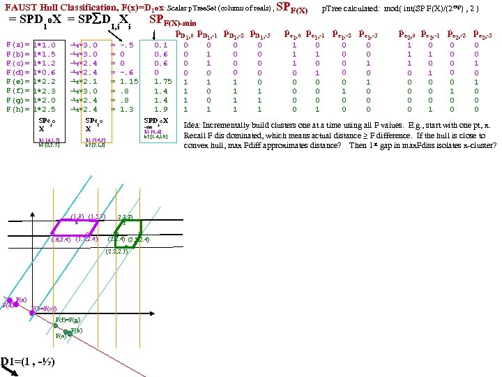
FAUST Hull Classification, F(x)=D 1 ox: Scalar p. Tree. Set (column of reals) , SPF(X) p. Tree calculated: mod( int(SP F(X)/(2 exp) , 2 ) = SPD 1 o. X = SP D 1, i. Xi SPF(X)-min p. D , 0 p. D , -1 p. D , -2 p. D , -3 pe , 0 pe , -1 pe , -2 pe F(a)= F(b)= F(c)= F(d)= F(e)= F(f)= F(g)= F(h)= 1*1. 0 1*1. 5 1*1. 2 1*0. 6 1*2. 2 1*2. 3 1*2. 0 1*2. 5 -½*3. 0 -½*2. 4 -½*2. 1 -½*3. 0 -½*2. 4 SPe 1 o X h 1 [2. 4, 3] h 2 [2. 1, 3] (1, 3) (1. 5, 3) b a c d (. 6, 2. 4) (1. 2, 2. 4) F(d) F(a) F(b=F(c)) F(f)=F(g) F(e) D 1=(1 , -½) F(h) 0. 1 0. 6 0 1. 75 1. 4 1. 9 -. 5 0 0 -. 6 1. 15. 8. 8 1. 3 SPe 2 o X h 1 [. 6, 1. 5] h 2 [2, 2. 5] = = = = SPD 1 o. X -mn h 1 [0, . 6] h 2 [1. 4, 1. 9] 2. 3, 3) f g h (2, 2. 4) (2. 5, 2. 4) e (2. 2, 2. 1) 1 0 0 1 1 1 0 1 0 0 1 1 1 0 0 0 1 1 1 1 0 0 0 1 0 1 0 0 0 1 0 0 1 0 0 0 2 1 1 1 0 0 0 2 0 1 0 0 2 0 0 1 0 0 0 2, -3 Idea: Incrementally build clusters one at a time using all F values. E. g. , start with one pt, x. Recall F dis dominated, which means actual distance ≥ F difference. If the hull is close to convex hull, max Fdiff approximates distance? Then 1 st gap in max. Fdiss isolates x-cluster?
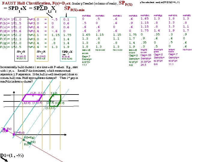
FAUST Hull Classification, F(x)=D 1 ox: Scalar p. Tree. Set (column of reals) , SPF(X) = SPD o. X = SP D X SPF(X)-min 1 1, i i mx. Fdf(a) F(a)= F(b)= F(c)= F(d)= F(e)= F(f)= F(g)= F(h)= 1*1. 0 1*1. 5 1*1. 2 1*0. 6 1*2. 2 1*2. 3 1*2. 0 1*2. 5 -½*3. 0 -½*2. 4 -½*2. 1 -½*3. 0 -½*2. 4 SPe 1 o. X SPe 2 o. X h 1 [. 6, 1. 5] h 2 [2, 2. 5] -. 5 0 0 -. 6 1. 15. 8. 8 1. 3 h 1 [2. 4, 3] h 2 [2. 1, 3] mx. Fdf(b) mx. Fdf(c) mx. Fdf(d) 0. 1 0. 6 0 1. 75 1. 4 1. 9 0. 5. 6. 6 1. 65 1. 3 1. 8 . 5 0. 6. 9 1. 15. 8. 8 1. 3 . 6. 6 0. 6 1. 15 1. 1. 8 1. 3 . 6. 9. 6 0 1. 75 1. 7 1. 4 1. 9 SPD 1 o. X = = = = {a, b, c, d} No b-core No c-core a-core. {a, b, c, d} d-core -mn h 1 [0, . 6] h 2 [1. 4, 1. 9] Incrementally build clusters 1 at a time with F values. E. g. , start with 1 pt, x. Recall F dis dominated, which means actual separation ≥ F separation. If the hull is well developed (close to convex hull) max Fdiff approximates distance? Then 1 st gap in max. Fdis isolates x-cluster? (1, 3) (1. 5, 3) b a c d (. 6, 2. 4) (1. 2, 2. 4) F(d) F(a) F(b=F(c)) F(f)=F(g) F(e) D 1=(1 , -½) F(h) p. Tree calculated: mod( int(SP F(X)/(2 exp) , 2 ) 2. 3, 3) f g h (2, 2. 4) (2. 5, 2. 4) e (2. 2, 2. 1) Gap=. 7 Density= 4/. 6^2= 11. 1 Gap=. 5 Density= 4/. 9^2= 4. 9 mx. Fdf(e) mx. Fdf(g) mx. Fdf(h) mx. Fdf(f) 1. 65 1. 15 1. 75 0. 9. 35. 3 1. 3. 8. 8 1. 4. 35. 6 0. 5 1. 8 1. 3 1. 9. 3. 6. 5 0 1. 3. 8 1. 1 1. 7. 9 0. 6. 6 {e, g, h} e-core {b, c, e, f, g, h} g-core {e, f, g, h} h-core No f-core Gap=. 5 Density= 6/. 8^2= 9. 4 Gap=. 7 Density= 4/. 6^2= 11. 1 Gap=. 55 Density= 3/. 35^2= 24. 5
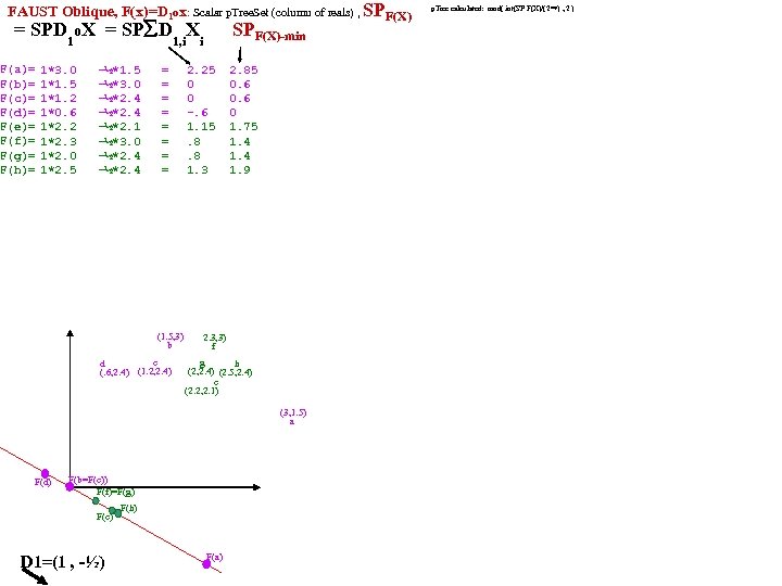
FAUST Oblique, F(x)=D 1 ox: Scalar p. Tree. Set (column of reals) , SPF(X) = SPD o. X = SP D X SPF(X)-min 1 F(a)= F(b)= F(c)= F(d)= F(e)= F(f)= F(g)= F(h)= 1*3. 0 1*1. 5 1*1. 2 1*0. 6 1*2. 2 1*2. 3 1*2. 0 1*2. 5 1, i -½*1. 5 -½*3. 0 -½*2. 4 -½*2. 1 -½*3. 0 -½*2. 4 = = = = (1. 5, 3) b c d (. 6, 2. 4) (1. 2, 2. 4) i 2. 25 0 0 -. 6 1. 15. 8. 8 1. 3 2. 85 0. 6 0 1. 75 1. 4 1. 9 2. 3, 3) f g h (2, 2. 4) (2. 5, 2. 4) e (2. 2, 2. 1) (3, 1. 5) a F(d) F(b=F(c)) F(f)=F(g) F(e) D 1=(1 , -½) F(h) F(a) p. Tree calculated: mod( int(SP F(X)/(2 exp) , 2 )
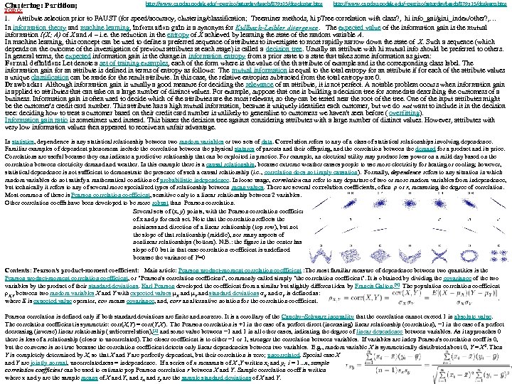
Clustering: Partition; http: //www. cs. ndsu. nodak. edu/~perrizo/saturday/teach/879 s 15/dmcluster. htm http: //www. cs. ndsu. nodak. edu/~perrizo/saturday/teach/879 s 15/dmlearn. htm TODO: 1. Attribute selection prior to FAUST (for speed/accuracy, clustering/classification; Treeminer methods, hi p. Tree correlation with class? , hi info_gai/gini_index/other? , … In information theory and machine learning, information gain is a synonym for Kullback–Leibler divergence. The expected value of the information gain is the mutual information I(X; A) of X and A – i. e. the reduction in the entropy of X achieved by learning the state of the random variable A. In machine learning, this concept can be used to define a preferred sequence of attributes to investigate to most rapidly narrow down the state of X. Such a sequence (which depends on the outcome of the investigation of previous attributes at each stage) is called a decision tree. Usually an attribute with hi mutual info should be preferred to others. In general terms, the expected information gain is the change in information entropy from a prior state to a state that takes some information as given: Formal definition: Let denote a set of training examples, each of the form where is the value of the th attribute of example and is the corresponding class label. The information gain for an attribute is defined in terms of entropy as follows: The mutual information is equal to the total entropy for an attribute if for each of the attribute values a unique classification can be made for the result attribute. In this case, the relative entropies subtracted from the total entropy are 0. Drawbacks: Although information gain is usually a good measure for deciding the relevance of an attribute, it is not perfect. A notable problem occurs when information gain is applied to attributes that can take on a large number of distinct values. For example, suppose that one is building a decision tree for some data describing the customers of a business. Information gain is often used to decide which of the attributes are the most relevant, so they can be tested near the root of the tree. One of the input attributes might be the customer's credit card number. This attribute has a high mutual information, because it uniquely identifies each customer, but we do not want to include it in the decision tree: deciding how to treat a customer based on their credit card number is unlikely to generalize to customers we haven't seen before ( overfitting). Information gain ratio is sometimes used instead. This biases the decision tree against considering attributes with a large number of distinct values. However, attributes with very low information values then appeared to receive an unfair advantage. In statistics, dependence is any statistical relationship between two random variables or two sets of data. Correlation refers to any of a class of statistical relationships involving dependence. Familiar examples of dependent phenomena include the correlation between the physical statures of parents and their offspring, and the correlation between the demand for a product and its price. Correlations are useful because they can indicate a predictive relationship that can be exploited in practice. For example, an electrical utility may produce less power on a mild day based on the correlation between electricity demand weather. In this example there is a causal relationship, because extreme weather causes people to use more electricity for heating or cooling; however, statistical dependence is not sufficient to demonstrate the presence of such a causal relationship (i. e. , correlation does not imply causation). Formally, dependence refers to any situation in which random variables do not satisfy a mathematical condition of probabilistic independence. In loose usage, correlation can refer to any departure of two or more random variables from independence, but technically it refers to any of several more specialized types of relationship between mean values. There are several correlation coefficients, often ρ or r, measuring the degree of correlation. Most common of these is Pearson correlation coefficient, sensitive only to a linear relationship between 2 variables. Other correlation coeffs have been developed to be more robust than Pearson correlation. Several sets of (x, y) points, with the Pearson correlation coefficient of x and y for each set. Note that the correlation reflects the noisiness and direction of a linear relationship (top row), but not the slope of that relationship (middle), nor many aspects of nonlinear relationships (bottom). N. B. : the figure in the center has a slope of 0 but in that case correlation coefficient is undefined because the variance of Y=0 Contents: Pearson's product-moment coefficient: Main article: Pearson product-moment correlation coefficient : The most familiar measure of dependence between two quantities is the Pearson product-moment correlation coefficient, or "Pearson's correlation coefficient", commonly called simply "the correlation coefficient". It is obtained by dividing the covariance of the two variables by the product of their standard deviations. Karl Pearson developed the coefficient from a similar but slightly different idea by Francis Galton. [4] The population correlation coefficient ρX, Y between two random variables X and Y with expected values μX and μY and standard deviations σX and σY is defined as: where E is expected value operator, cov means covariance, and, corr an alternative notation for the correlation coefficient. Pearson correlation is defined only if both standard deviations are finite and nonzero. It is a corollary of the Cauchy–Schwarz inequality that the correlation cannot exceed 1 in absolute value. The correlation coefficient is symmetric: corr(X, Y) = corr(Y, X). The Pearson correlation is +1 in the case of a perfect direct (increasing) linear relationship (correlation), − 1 in the case of a perfect decreasing (inverse) linear relationship (anticorrelation), [5] and some value between − 1 and 1 in all other cases, indicating the degree of linear dependence between variables. As it approaches 0 there is less of a relationship (closer to uncorrelated). The closer coefficient is to either − 1 or 1, stronger the correlation between variables. If variables are indep Pearson's correlation coeff is 0, but the converse is not true because the correlation coefficient detects only linear dependencies between two variables. E. g. , random variable X is symmetrically distributed about 0, Y = X 2. Then Y is completely determined by X, so that X and Y are perfectly dependent, but their correlation is zero; uncorrelated. Special case X and Y are jointly normal, uncorrelatedness = independence. If a series of n measmnts of X , Y written xi and yi i = 1. . . n, sample correlation coefficient can be used to estimate pop Pearson correlation r between X and Y. Sample correlation coeff is written where x and y are the sample means of X and Y, and sx and sy are the sample standard deviations of X and Y.
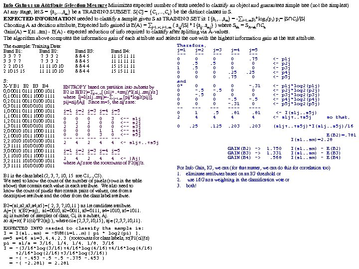
Info Gain as an Attribute Selection Measure Minimizes expected number of tests needed to classify an object and guarantees simple tree (not the simplest) At any stage, let S = {s 1, . . . , sm} be a TRAINING SUBSET. S[C] = {C 1, . . . , Cc} be the distinct classes in S. EXPECTED INFORMATION needed to classify a sample given S as TRAINING SET is: I{s 1, . . . , sm} = -∑i=1. . mpi*log 2(pi) pi= |S∩Ci|/|S| Choosing A as decision attribute, Expected Info gained is E(A) = ∑j=1. . v; i=1. . m ( si, j/|S| * I{sij. . smj} ) where Skh = SA=ak∩Ch Gain(A) = I(s 1. . sm) - E(A) - expected reduction of info required to classify after splitting via A-values. The algorithm above computes the information gain of each attribute and selects the one with the highest information gain as the test attribute. The example: Training Data: Band B 1: Band B 2: 3 3 7 7 7 3 3 2 2 2 10 15 11 11 10 10 2 10 15 15 11 11 10 10 S: X-Y B 1 B 2 B 3 B 4 0, 0 0011 0111 1000 1011 0, 1 0011 1000 1111 0, 2 0111 0011 0100 1011 0, 3 0111 0010 0101 1011 1, 0 0011 0111 1000 1011 1, 1 0011 1000 1011 1, 2 0111 0011 0100 1011 1, 3 0111 0010 0101 1011 2, 0 0010 1011 1000 1111 2, 1 0010 1011 1000 1111 2, 2 1010 0100 1011 2, 3 1111 1010 0100 1011 3, 0 0010 1011 1000 1111 3, 1 1010 1011 1000 1111 3, 2 1111 1010 0100 1011 3, 3 1111 1010 0100 1011 Band B 3: 8 8 4 5 8 8 4 4 Band B 4: 11 15 11 11 11 15 15 11 11 ENTROPY based on partition into subsets by B 2 is E(B 2)= j=1. . v[ (s 1 j+. . +smj)*I(s 1 j. . smj)/s ] where Ij=I(s 1 j. . smj)=- i=1. . m [pij*log 2(pij)], pij=sij/|Aj| Since m=5, the sij's are: j=1 j=2 j=3 j=4 j=5 --- --- --0 0 3 <-- s 1 j 0 2 2 0 0 <-- s 2 j 2 2 0 0 0 <-- s 3 j 0 0 0 1 1 <-- s 4 j 0 0 0 3 0 <-- s 5 j --- --- --2 4 4 <- s 1 j+. . +s 5 j j=1 j=2 j=3 j=4 j=5 --- --- --2 4 4 <- |Aj| where Aj's are the rootcounts of P 2(aj)'s. B 1 is the class label (2, 3, 7, 10, 15 are C 1, . . , C 5). We need to know the count of the number of pixels (rows in the table above) that contain each value in each attribute. We also need to know the count of pixels that contain pairs of values, one from a descriptive attribute and the other from the class label attribute. B 2=(a 1, a 2, a 3, a 4, a 5}={ 2, 3, 7, 10, 11 } as 1 st candidate attribute. Aj={t: : t(B 2)=aj}, a 1=0010, a 2=0011, a 3=0111, a 4=1010, a 5=1011. sij is number of samples of class, Ci, in a subset, Aj. so sij=rc( P 1(ci)^P 2(aj) ), where ci {2, 3, 7, 10, 15}, aj {2, 3, 7, 10, 11}. EXPECTED INFO needed to classify the sample is: I = I(s 1. . sm) = -SUM(i=1. . m)[ pi * log 2(pi) ], m=5 s=16 si=3, 4, 4, 2, 3 (rootcounts for class labels, rc(P 1(ci))'s) pi = s 1/s = 3/16, 1/4, 1/8, 3/16 I = -(3/16*log(3/16)+4/16*log(4/16) +2/16*log(2/16)+3/16*log(3/16)) = -( -. 453 -. 5 -. 375 -. 453 ) = -( -2. 281) = 2. 281 Therefore, j=1 j=2 j=3 ------0 0 0 0. 5. 5 1. 5 0 0 0 0 and 0* 0 0 0 -. 5 0 0 0 0 -----0 1. 5 2 4 4 0 . 25 . 125 j=4 --0 0 0. 25. 75 j=5 --. 75 0 0. 25 0 <<<<<- p 1 j p 2 j p 3 j p 4 j p 5 j p 1 j*log 2(p 1 j) p 2 j*log 2(p 2 j) p 3 j*log 2(p 3 j) p 4 j*log 2(p 4 j) p 5 j*log 2(p 5 j) 0 0 0 -. 5 -. 31 ---. 81 4 -. 31 0 0 -. 5 0 ---. 81 4 <<<<<- . 203 (s 1 j+. . +s 5 j)*I(s 1 j. . s 5 j)/16 <- I(s 1 j. . s 5 j) <- s 1 j+. . +s 5 j so that, E(B 2)=. 781 I(s 1. . sm)=2. 28 GAIN(B 2) -> GAIN(B 3) -> GAIN(B 4) -> 1. 750 1. 331. 568 I(s 1. . sm) - E(B 2) I(s 1. . sm) - E(B 3) I(s 1. . sm) - E(B 4) For Info Gain, IG, we can (for that matter, we can do this for correlation too) 1. eliminate attributes based on an IG threshold or 2. use 1/IG as a weighting in the classification vote or 3. both!
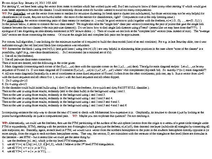
From: Arjun Roy January 14, 2015 2: 03 AM For starting 'd', we have been using the vector from mean to median which has worked quite well. But I am curious to know if there is any other starting 'd' which would give even better separation between the classes. I could randomly choose some d's but also wanted to avoid too many computations. WP: For clustering, we use the vector from mean to median for recursive clustering (to break apart a cluster into subclusters), but those vectors may not be very helpful for classification (of course, they are not hurtful either - the more d's the merrier for classification, right? Computation cost is the only limiting issue. ) For classification, the vectors connecting pairs of class means (or medians or. . . ) would be good vectors to pick (together with the freebees, e 1=(1. 0. . . 0), . . . , en=(0. . . 0, 1) ). In the picture below, d seems to connect the two class means? We might also take the "single link" class pair vectors (connecting the pair of points that give the single link distance between the two classes (=the min pairwise distance)). Do we know how to find single link distance using p. Trees? (seems like we may have done that? ? ). I apologize if I am forgetting an idea already mentioned in MY lecture slides. ; -) Then of course we can look at the "complete link" vectors (max instead of min). The "average link" vectors are those connecting the means. Of course the single link and complete link pairs can be approximate. For convex hull algorithm, I was looking for the minimum number of d required to build the class model (kind of an end condition). For e. g. in last Saturday slide, one d was sufficient enough (the red line) and black line computation was redundant. WP: Remember the black ( using d=e 2=(0, 1) )and gold lines ( using d=e 1=(1, 0) ) are very helpful in eliminating false positives in the case where "none of the classes" is a possibility, right? (e. g. , one-classification). . So I recommend (as a minimal set of d's): 1. Use all ei (the freebees). 2. Use all pairwise class mean connectors. Then if more are desired, add the following in the order given: 3. Main diagonals (connecting each corner of the (0, x 2, . . . , xn) face with the opposite corner on the (1, x 2, . . . , xn) face). The alg for main diagonal endpts: Let x 2, . . . , xn be any sequence of 0's and 1's. D is a main diagonal iff D connects (0, x 2, x 3, . . . , xn) to (1, x 2', x 3', . . . , xn') where ' =bit complement (flip each bit). So exactly 2^(n-1) main diagonals? ? 4. All non-main diagonals (basically fix a set of coordinates at some fixed sequence of 0's and 1's then from the other coordinates, pick one, say k. Run a vector from xk=0 with the fixed sequence and all others 0 or 1, to xk=1 with the fixed sequence and all others flipped. 5. Do 3 using xh=1/2 6. Do 4 using xh=1/2 So the classifier could build initial hulls using 1 first (Use only the freebees , for a quick and dirty FAUST HULL classifier. ). Then as the user is using those results, reclassify (add to the class hulls) in the background using 1 and 2. Then as the user is using those results, reclassify in the background using 1 and 2 and 3 and 4 and 5 and 6 Is computing variance the only way to choose the next d? I need to check with Mohammad how expensive it is. Graphically, its intuitive to choose d just by looking at the points but algorithmically its quite a computational pain. WP: Maybe you can re-phrase this question? I'm not catching it. WP: Alternatively, we could use the freebees, then use the PTM partitioning of the surface of the unit sphere (vectors from the origin to a vertex of a great circle triangle under PTM or equivalently, HTM), starting with the partition into 8 triangles (which gives just the feebees, e 1, e 2, e 3), then descend one layer (subdivide all triangles by connecting all side midpoints, etc. Basically, again, at each level in PTM, we would run a vector from the northern hemisphere to the point in the southern hemisphere directly opposite it (or more simply, from the origin to each northern hemisphere vertex. That way, the vectors, D, are coincident with the vertexes of the triangles at that level (there are formulas in the literatire – see HTM – but it seems like we could get the same thing by: 1. use the freebees {e 1. . en}, which is the top level PTM triangulation. 2. use all V 1={ ei ej | i=1, 2, 3; i j=2, 3}, which I believe is the 2 nd level PTM triangulation. 3. use all V 2={ v + w | v , w in V 1}, 4. use all V 3={ v + w | v , w in V 2}, …
25792ae2e3a5a05094a0a41c5ee8280b.ppt