

b8da4e95eaa4cfc9b6bf6cb706644397.ppt
- Количество слайдов: 59
 TNI: Computational Neuroscience Instructors: Peter Latham Maneesh Sahani Peter Dayan TA: Website: Phillipp Hehrmann, hehrmann@gatsby. ucl. ac. uk http: //www. gatsby. ucl. ac. uk/~hehrmann/TN 1/ (slides will be on website) Lectures: Review: Tuesday/Friday, 11: 00 -1: 00. Friday, 1: 00 -3: 00. Homework: Assigned Friday, due Friday (1 week later). first homework: 2 weeks later (no class Oct. 12).
 What is computational neuroscience? Our goal: figure out how the brain works.
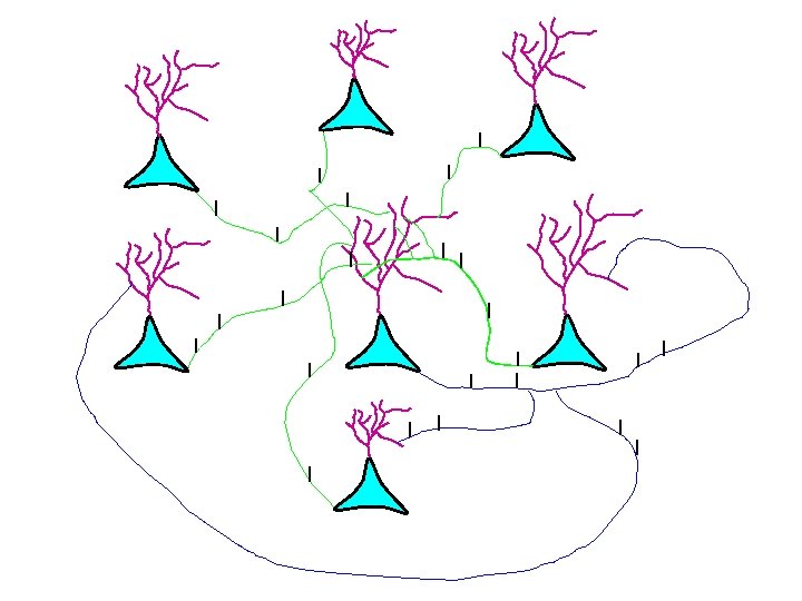
 There about 10 billion cubes of this size in your brain! 10 microns
") How do we go about making sense of this mess? David Marr (1945 -1980) proposed three levels of analysis: 1. the problem (computational level) 2. the strategy (algorithmic level) 3. how it’s actually done by networks of neurons (implementational level)
How do we go about making sense of this mess? David Marr (1945 -1980) proposed three levels of analysis: 1. the problem (computational level) 2. the strategy (algorithmic level) 3. how it’s actually done by networks of neurons (implementational level)
: 2 -D image on retina → 3 -D") Example #1: vision. the problem (Marr): 2 -D image on retina → 3 -D reconstruction of a visual scene.
Example #1: vision. the problem (Marr): 2 -D image on retina → 3 -D reconstruction of a visual scene.
: 2 -D image on retina → reconstruction") Example #1: vision. the problem (modern version): 2 -D image on retina → reconstruction of latent variables. house sun tree bad artist
Example #1: vision. the problem (modern version): 2 -D image on retina → reconstruction of latent variables. house sun tree bad artist
: 2 -D image on retina → reconstruction") Example #1: vision. the problem (modern version): 2 -D image on retina → reconstruction of latent variables. the algorithm: graphical models. x 1 r 1 x 2 r 2 ^1 x x 3 r 3 ^2 x latent variables r 4 ^3 x peripheral spikes estimate of latent variables
Example #1: vision. the problem (modern version): 2 -D image on retina → reconstruction of latent variables. the algorithm: graphical models. x 1 r 1 x 2 r 2 ^1 x x 3 r 3 ^2 x latent variables r 4 ^3 x peripheral spikes estimate of latent variables
: 2 -D image on retina → reconstruction") Example #1: vision. the problem (modern version): 2 -D image on retina → reconstruction of latent variables. the algorithm: graphical models. implementation in networks of neurons: no clue.
Example #1: vision. the problem (modern version): 2 -D image on retina → reconstruction of latent variables. the algorithm: graphical models. implementation in networks of neurons: no clue.
 Example #2: memory. the problem: recall events, typically based on partial information.
 Example #2: memory. the problem: recall events, typically based on partial information. associative or content-addressable memory. the algorithm: dynamical systems with fixed points. r 3 r 2 r 1 activity space
 Example #2: memory. the problem: recall events, typically based on partial information. associative or content-addressable memory. the algorithm: dynamical systems with fixed points. neural implementation: Hopfield networks. xi = sign( ∑j Jij xj)
 Comment #1: the problem: the algorithm: neural implementation:
 Comment #1: the problem: the algorithm: neural implementation: easier harder often ignored!!!
 Comment #1: the problem: the algorithm: neural implementation: easier harder My favorite example: CPGs (central pattern generators) rate
 Comment #2: the problem: the algorithm: neural implementation: easier harder You need to know a lot of math!!!!! x 1 r 1 x 2 r 2 ^1 x r 3 ^2 x r 3 x 3 r 4 ^3 x r 2 r 1 activity space
 Comment #3: the problem: the algorithm: neural implementation: easier harder This is a good goal, but it’s hard to do in practice. We shouldn’t be afraid to just mess around with experimental observations and equations.
 A classic example: Hodgkin and Huxley. dendrites soma axon voltage +40 m. V 1 ms time -50 m. V 100 ms
 – g.") A classic example: Hodgkin and Huxley. C d. V/dt = –g. L(V-VL) – g. Nam 3 h(V-VNa) – … dm/dt = … …
A classic example: Hodgkin and Huxley. C d. V/dt = –g. L(V-VL) – g. Nam 3 h(V-VNa) – … dm/dt = … …
 the problem: the algorithm: neural implementation: easier harder A lot of what we do as computational neuroscientists is turn experimental observations into equations. The goal here is to understand how networks or single neurons work. We should always keep in mind that: a) this is less than ideal, b) we’re really after the big picture: how the brain works.
 Basic facts about the brain
 Your brain
 6 layers ~30 cm ~0. 5 cm subcortical structures") Your cortex unfolded neocortex (cognition) 6 layers ~30 cm ~0. 5 cm subcortical structures (emotions, reward, homeostasis, much more)
Your cortex unfolded neocortex (cognition) 6 layers ~30 cm ~0. 5 cm subcortical structures (emotions, reward, homeostasis, much more)
 Your cortex unfolded 1 cubic millimeter, ~3*10 -5 oz
") 1 mm 3 of cortex: 50, 000 neurons 10000 connections/neuron (=> 500 million connections) 4 km of axons
1 mm 3 of cortex: 50, 000 neurons 10000 connections/neuron (=> 500 million connections) 4 km of axons
 1 mm 3 of cortex: 1 mm 2 of a CPU: 50, 000 neurons 10000 connections/neuron (=> 500 million connections) 4 km of axons 1 million transistors 2 connections/transistor (=> 2 million connections). 002 km of wire
 1 mm 3 of cortex: 1 mm 2 of a CPU: 50, 000 neurons 10000 connections/neuron (=> 500 million connections) 4 km of axons 1 million transistors 2 connections/transistor (=> 2 million connections). 002 km of wire whole brain (2 kg): whole CPU: 1011 neurons 1015 connections 8 million km of axons 109 transistors 2*109 connections 2 km of wire
 1 mm 3 of cortex: 1 mm 2 of a CPU: 50, 000 neurons 10000 connections/neuron (=> 500 million connections) 4 km of axons 1 million transistors 2 connections/transistor (=> 2 million connections). 002 km of wire whole brain (2 kg): whole CPU: 1011 neurons 1015 connections 8 million km of axons 109 transistors 2*109 connections 2 km of wire
 soma (spike generation) axon (output) voltage +40 m. V 1 ms time") dendrites (input) soma (spike generation) axon (output) voltage +40 m. V 1 ms time -50 m. V 100 ms
dendrites (input) soma (spike generation) axon (output) voltage +40 m. V 1 ms time -50 m. V 100 ms
 synapse current flow
 synapse current flow
 voltage +40 m. V -50 m. V time 100 ms
 neuron i neuron j V on neuron i neuron j emits a spike: EPSP t 10 ms
 neuron i neuron j V on neuron i neuron j emits a spike: IPSP t 10 ms
 neuron i neuron j V on neuron i neuron j emits a spike: IPSP t 10 ms amplitude = wij
 neuron i neuron j V on neuron i neuron j emits a spike: IPSP t 10 ms changes with learning amplitude = wij
 synapse current flow
 A bigger picture view of the brain
 x r latent variables peripheral spikes sensory processing ^ r action selection emotions cognition memory ^ r' “direct” code for latent variables brain “direct” code for motor actions motor processing r' peripheral spikes x' motor actions
 r
r
 r
r
 r
r
 r
r
 you are the cutest stick figure ever! r
 x action selection emotions cognition memory r ^ r' r' brain x' Questions: 1. How does the brain re-represent latent variables? 2. How does it manipulate re-represented variables? 3. How does it learn to do both? Ask at three levels: 1. What are the properties of task x? 2. What are the algorithms? 3. How are they implemented in neural circuits?
 Knowing the algorithms is a critical, but often neglected, step!!! We know the algorithms that the vestibular system uses. We know (sort of) how it’s implemented at the neural level. We know the algorithm for echolocation. We know (mainly) how it’s implemented at the neural level. We know the algorithm for computing x+y. We know (mainly) how it might be implemented in the brain.
 Knowing the algorithms is a critical, but often neglected, step!!! We don’t know the algorithms for anything else. We don’t know how anything else is implemented at the neural level. This is not a coincidence!!!!
 ed s ia b What we know about the brain y H ig l h
 1. Anatomy. We know a lot about what is where. But be careful about labels: neurons in motor cortex sometimes respond to color. Connectivity. We know (more or less) which area is connected to which. We don’t know the wiring diagram at the microscopic level. wij
.") 2. Single neurons. We know very well how point neurons work (think Hodgkin Huxley). Dendrites. Lots of potential for incredibly complex processing. My guess: they make neurons bigger and reduce wiring length.
2. Single neurons. We know very well how point neurons work (think Hodgkin Huxley). Dendrites. Lots of potential for incredibly complex processing. My guess: they make neurons bigger and reduce wiring length.
 3. The neural code. We’re pretty sure that information is carried in action potentials. We’re not sure what aspects of action potentials carry the information. The two main candidates: precise timing firing rate Once you get away from periphery, it’s mainly firing rate.
 4. Recurrent networks of spiking neurons. This is a field that is advancing rapidly! There were two absolutely seminal papers about a decade ago: van Vreeswijk and Sompolinsky (Science, 1996) van Vreeswijk and Sompolinsky (Neural Comp. , 1998) We now understand very well randomly connected networks (harder than you might think), and (I believe) we are on the verge of: i) understanding networks that have interesting computational properties. ii) computing the correlational structure in those networks.
, but it’s not") 5. Learning. We know a lot of facts (LTP, LTD, STDP), but it’s not clear which, if any, are relevant. Theorists are starting to develop unsupervised learning algorithms, mainly ones that maximize mutual information. These are promising, but the link to the brain has not been fully established.
5. Learning. We know a lot of facts (LTP, LTD, STDP), but it’s not clear which, if any, are relevant. Theorists are starting to develop unsupervised learning algorithms, mainly ones that maximize mutual information. These are promising, but the link to the brain has not been fully established.
: You have about 1015 synapses. If it") A word about learning (remember these numbers!!!): You have about 1015 synapses. If it takes 1 bit of information to set a synapse, you need 1015 bits to set all of them. 30 years ≈ 109 seconds. To set 1/10 of your synapses in 30 years, you must absorb 100, 000 bits/second. Learning in the brain is almost completely unsupervised!!!
A word about learning (remember these numbers!!!): You have about 1015 synapses. If it takes 1 bit of information to set a synapse, you need 1015 bits to set all of them. 30 years ≈ 109 seconds. To set 1/10 of your synapses in 30 years, you must absorb 100, 000 bits/second. Learning in the brain is almost completely unsupervised!!!
. Vestibular system,") 6. Where we know algorithms we know the neural implementation (sort of). Vestibular system, sound localization, echolocation, x+y.
6. Where we know algorithms we know the neural implementation (sort of). Vestibular system, sound localization, echolocation, x+y.
. a. Anatomy. b. Single neurons. c.") 1. What we know: my score (1=low, 10=high). a. Anatomy. b. Single neurons. c. The neural code. d. Recurrent networks of spiking neurons. e. Learning. 7 7 5 4 2 Questions: all answers are “we don’t know”. 1. How does the brain re-represent latent variables? 2. How does it manipulate re-represented variables? 3. How does it learn to do both? 0. 001 0. 002 0. 001
1. What we know: my score (1=low, 10=high). a. Anatomy. b. Single neurons. c. The neural code. d. Recurrent networks of spiking neurons. e. Learning. 7 7 5 4 2 Questions: all answers are “we don’t know”. 1. How does the brain re-represent latent variables? 2. How does it manipulate re-represented variables? 3. How does it learn to do both? 0. 001 0. 002 0. 001
 Outline: 1. 2. 3. 4. Basics: single neurons/axons/dendrites/synapses. Language of neurons: neural coding. What we know about networks (very little). Learning at network and behavioral level. Latham Sahani Latham Dayan
: 1. 2. 3. 4. 5. What") Outline for this part of the course (biophysics): 1. 2. 3. 4. 5. What makes a neuron spike. How current propagates in dendrites. How current propagates in axons. How synapses work. Lots and lots of math!!!
Outline for this part of the course (biophysics): 1. 2. 3. 4. 5. What makes a neuron spike. How current propagates in dendrites. How current propagates in axons. How synapses work. Lots and lots of math!!!