Timed Automata II CS 5270 Lecture 5 17

Timed Automata II CS 5270 Lecture 5 17. 02. 05 Lecture 5 1

Goals • Timed Transition Systems: – Review – Definition – Timed behaviors. – Parallel composition – Reachability • UPPAAL 17. 02. 05 Lecture 5 2

Timed Transition Systems • Timed Transition Systems = Transition Systems + Clock Variables. • Clock variables. – – Used to record the passage of (real) time. Act like Timers. Can be read. Transitions constrained (guarded) by current values of clock variables. – Can be reset to 0 during a transition. q Continue to evolve (in real time) until reset. 17. 02. 05 Lecture 5 3

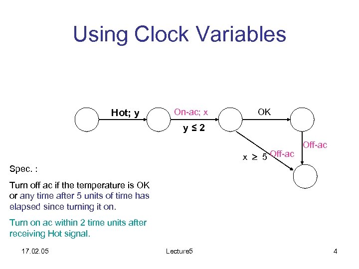Using Clock Variables Hot; y On-ac; x OK y≤ 2 x 5 Off-ac Spec. : Turn off ac if the temperature is OK or any time after 5 units of time has elapsed since turning it on. Turn on ac within 2 time units after receiving Hot signal. 17. 02. 05 Lecture 5 4

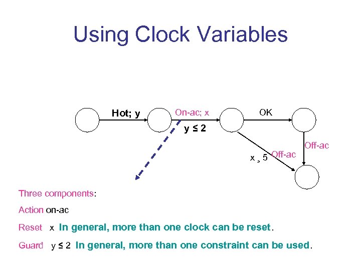Using Clock Variables Hot; y On-ac; x OK y≤ 2 x ¸ 5 Off-ac Three components: Action on-ac Reset x In general, more than one clock can be reset. Guard y ≤ 2 In general, more than one constraint can be used.

State Invariants • A clock constraint is associated with each state: state invariant – The system can stay in the state only as long as the state’s invariant is not violated. • For time points which violate the invariant one expects an output transition to be enabled. – Otherwise a time deadlock. q The progress of time is blocked (in the model!). 17. 02. 05 Lecture 5 6

Timed Transition Systems: Definition • Clock Constraints: • X, a finite set of clocks (clock variables). – x X • (X), the set of clock constraints over X. – (X) = x ≤ c | x ≥ c | x < c | x >c | 1 2 | –c Q q Q , the set of non-negative rational numbers. • 2 X --- The set of subsets of X q X = {x, y} 2 X = { , {x}, {y}, {x, y} } 17. 02. 05 Lecture 5 7

Timed Transition Systems • TTS = (S, sin, Act, X, I, ) – S is a finite set of states. – sin, initial state – Act, a finite set of actions – X, a finite set of clock variables. –I: S (X), assigns a clock invariant to each state. – S Act 2 X (X) S , the transition relation. 17. 02. 05 Lecture 5 8

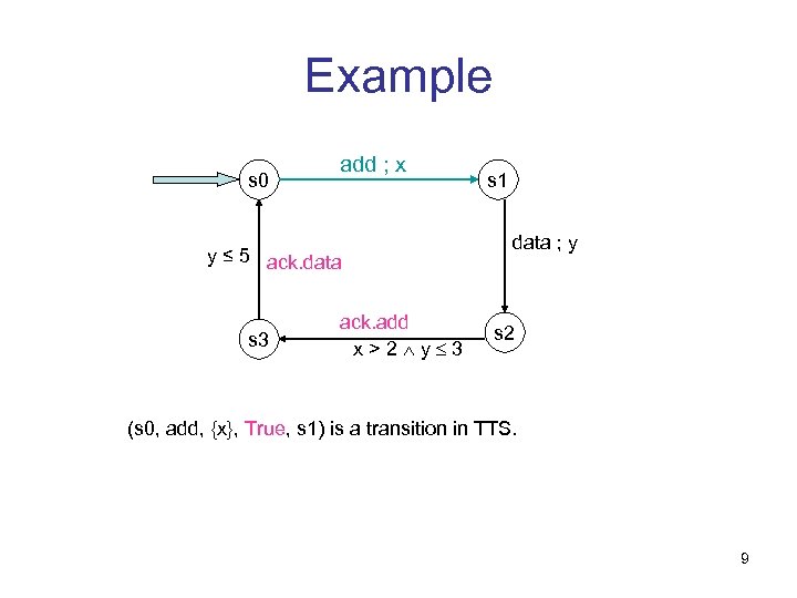Example s 0 add ; x y ≤ 5 ack. data s 3 ack. add x>2 y 3 s 1 data ; y s 2 (s 0, add, {x}, True, s 1) is a transition in TTS. 9

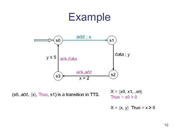Example s 0 add ; x y ≤ 5 ack. data s 3 ack. add x>2 (s 0, add, {x}, True, s 1) is a transition in TTS. s 1 data ; y s 2 X = {x 0, x 1, . . xn} True = x 0 ≥ 0 X = {x, y} True = x 0 10

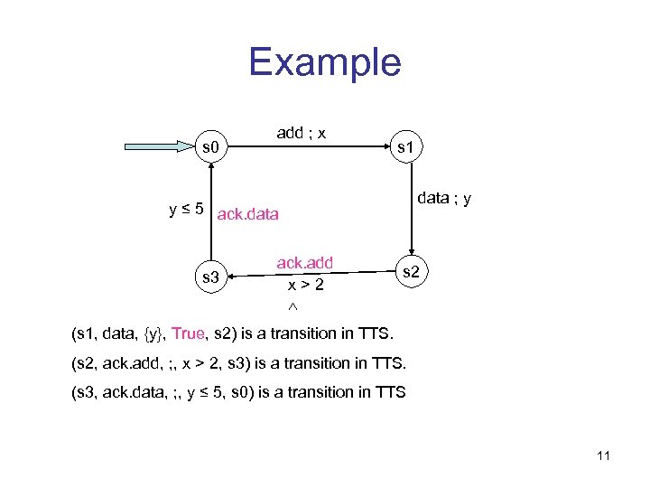Example s 0 add ; x s 1 data ; y y ≤ 5 ack. data s 3 ack. add x>2 s 2 (s 1, data, {y}, True, s 2) is a transition in TTS. (s 2, ack. add, ; , x > 2, s 3) is a transition in TTS. (s 3, ack. data, ; , y ≤ 5, s 0) is a transition in TTS 11

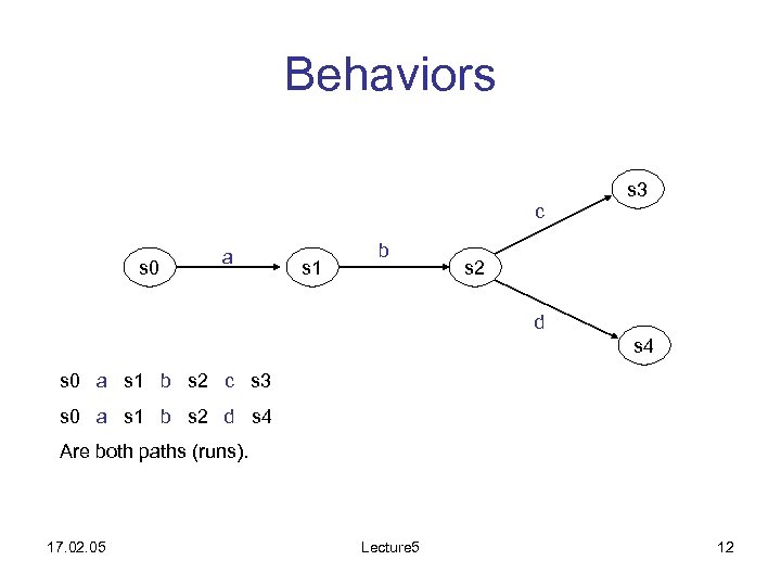Behaviors s 3 c s 0 a s 1 b s 2 d s 4 s 0 a s 1 b s 2 c s 3 s 0 a s 1 b s 2 d s 4 Are both paths (runs). 17. 02. 05 Lecture 5 12

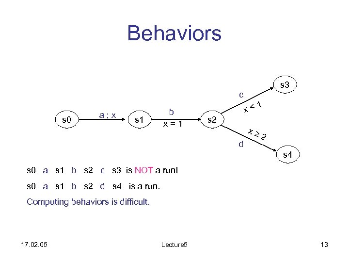Behaviors s 3 c s 0 a; x s 1 b x=1 x< s 2 1 x≥ d 2 s 4 s 0 a s 1 b s 2 c s 3 is NOT a run! s 0 a s 1 b s 2 d s 4 is a run. Computing behaviors is difficult. 17. 02. 05 Lecture 5 13

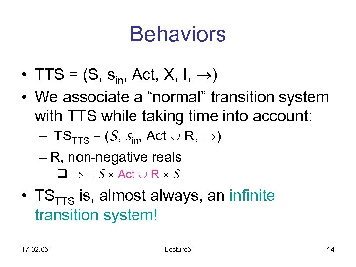Behaviors • TTS = (S, sin, Act, X, I, ) • We associate a “normal” transition system with TTS while taking time into account: – TSTTS = (S, sin, Act R, ) – R, non-negative reals q S Act R S • TSTTS is, almost always, an infinite transition system! 17. 02. 05 Lecture 5 14

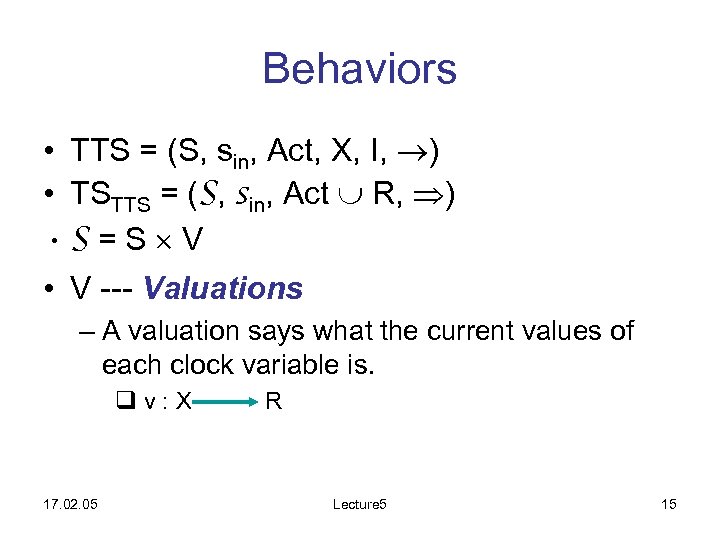Behaviors • TTS = (S, sin, Act, X, I, ) • TSTTS = (S, sin, Act R, ) • S=S V • V --- Valuations – A valuation says what the current values of each clock variable is. qv: X 17. 02. 05 R Lecture 5 15

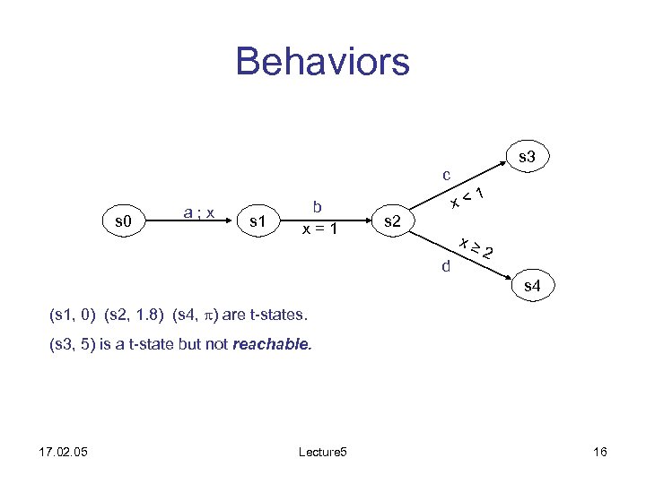Behaviors s 3 c s 0 a; x s 1 b x=1 x< s 2 1 x≥ d 2 s 4 (s 1, 0) (s 2, 1. 8) (s 4, ) are t-states. (s 3, 5) is a t-state but not reachable. 17. 02. 05 Lecture 5 16

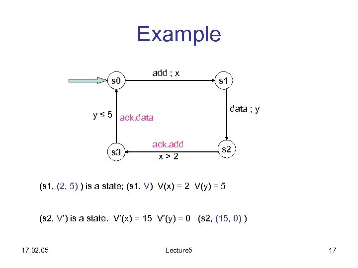Example s 0 add ; x s 1 data ; y y ≤ 5 ack. data s 3 ack. add x>2 s 2 (s 1, (2, 5) ) is a state; (s 1, V) V(x) = 2 V(y) = 5 (s 2, V’) is a state. V’(x) = 15 V’(y) = 0 (s 2, (15, 0) ) 17. 02. 05 Lecture 5 17

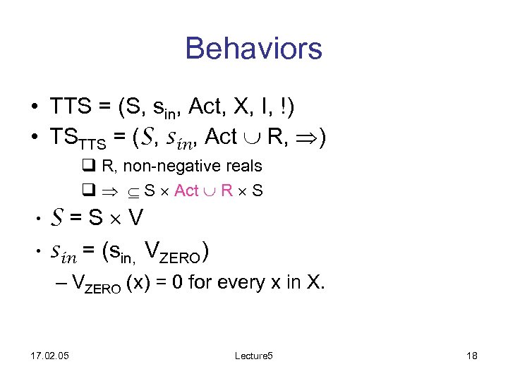Behaviors • TTS = (S, sin, Act, X, I, !) • TSTTS = (S, sin, Act R, ) q R, non-negative reals q S Act R S • S=S V • sin = (sin, VZERO) – VZERO (x) = 0 for every x in X. 17. 02. 05 Lecture 5 18

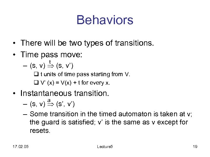Behaviors • There will be two types of transitions. • Time pass move: t – (s, v) (s, v’) q t units of time pass starting from V. q V’ (x) = V(x) + t for every x. • Instantaneous transition. a – (s, v) (s’, v’) – Some transition in the timed automaton is taken at v; the guard is satisfied; v’ is the same as v except for resets. 17. 02. 05 Lecture 5 19

Example s 0 add ; x y ≤ 5 ack. data s 3 (s 1, (0, 5)) 1 ack. add x>2 s 1 data ; y s 2 (s 2, (1, 6) ) Time- passing move? 20

Example s 0 add ; x y ≤ 5 ack. data s 3 (s 1, (0, 5)) 1 ack. add x>2 s 1 data ; y s 2 (s 1, (1, 7) ) Time- passing move? 21

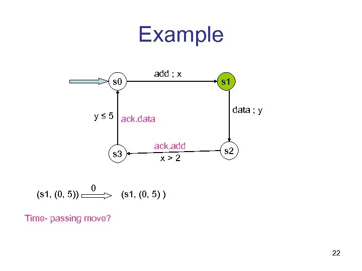Example s 0 add ; x y ≤ 5 ack. data s 3 (s 1, (0, 5)) 0 ack. add x>2 s 1 data ; y s 2 (s 1, (0, 5) ) Time- passing move? 22

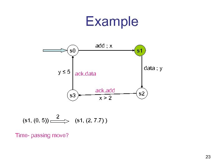Example s 0 add ; x y ≤ 5 ack. data s 3 (s 1, (0, 5)) 2 ack. add x>2 s 1 data ; y s 2 (s 1, (2, 7. 7) ) Time- passing move? 23

Example s 0 add ; x data ; y y ≤ 5 ack. data s 3 (s 0, (3, 3) ) add s 1 ack. add x>2 (s 1, (0, 3)) s 2 a transition in TS? 24

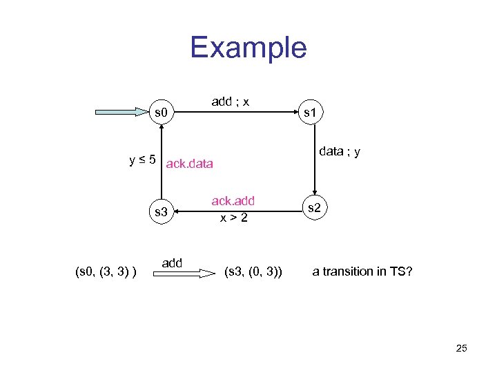Example s 0 add ; x data ; y y ≤ 5 ack. data s 3 (s 0, (3, 3) ) add s 1 ack. add x>2 (s 3, (0, 3)) s 2 a transition in TS? 25

Example s 0 add ; x data ; y y ≤ 5 ack. data s 3 (s 0, (3, 3) ) add s 1 ack. add x>2 (s 1, (0, 4)) s 2 a transition in TS? 26

Example s 0 add ; x data ; y y ≤ 5 ack. data s 3 (s 0, (0, 0) ) add s 1 ack. add x>2 (s 1, (0, 0)) s 2 a transition in TS? 27

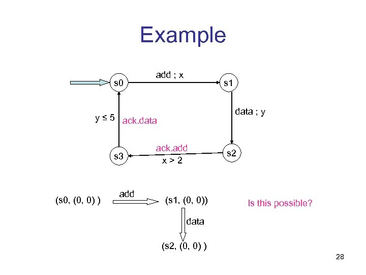Example s 0 add ; x s 1 data ; y y ≤ 5 ack. data s 3 (s 0, (0, 0) ) add ack. add x>2 (s 1, (0, 0)) s 2 Is this possible? data (s 2, (0, 0) ) 28

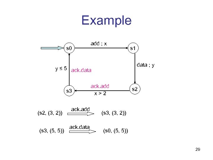Example s 0 add ; x data ; y y ≤ 5 ack. data s 3 (s 2, (3, 2)) (s 3, (5, 5)) ack. add ack. data s 1 ack. add x>2 s 2 (s 3, (3, 2)) (s 0, (5, 5)) 29

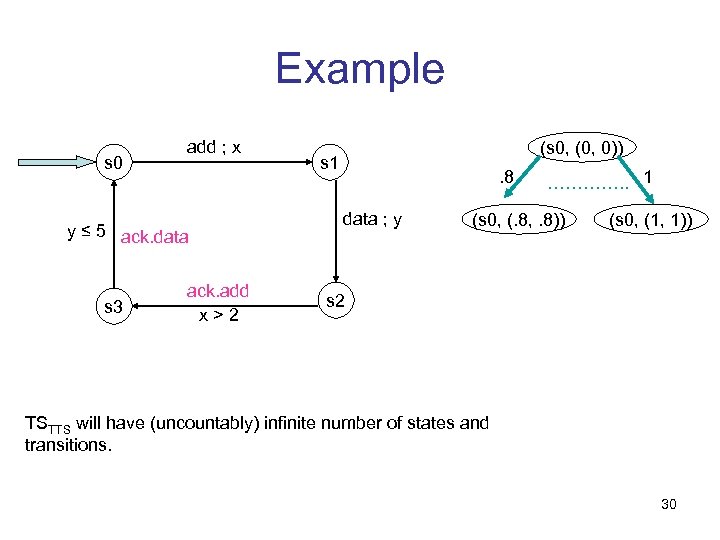Example s 0 add ; x y ≤ 5 ack. data s 3 ack. add x>2 (s 0, (0, 0)) s 1 . 8 data ; y …………. . 1 (s 0, (. 8, . 8)) (s 0, (1, 1)) s 2 TSTTS will have (uncountably) infinite number of states and transitions. 30

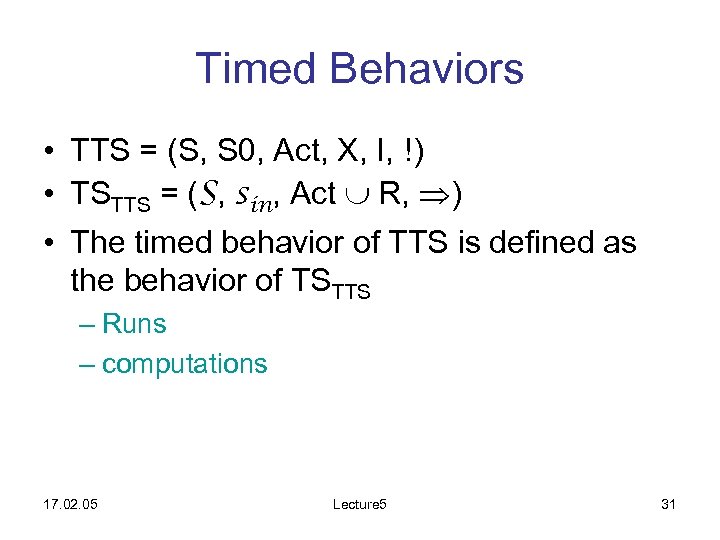Timed Behaviors • TTS = (S, S 0, Act, X, I, !) • TSTTS = (S, sin, Act R, ) • The timed behavior of TTS is defined as the behavior of TSTTS – Runs – computations 17. 02. 05 Lecture 5 31

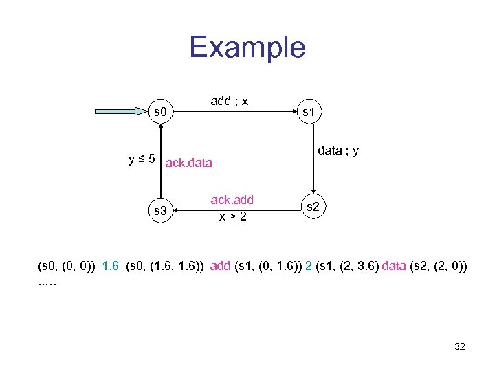Example s 0 add ; x y ≤ 5 ack. data s 3 ack. add x>2 s 1 data ; y s 2 (s 0, (0, 0)) 1. 6 (s 0, (1. 6, 1. 6)) add (s 1, (0, 1. 6)) 2 (s 1, (2, 3. 6) data (s 2, (2, 0)). . … 32

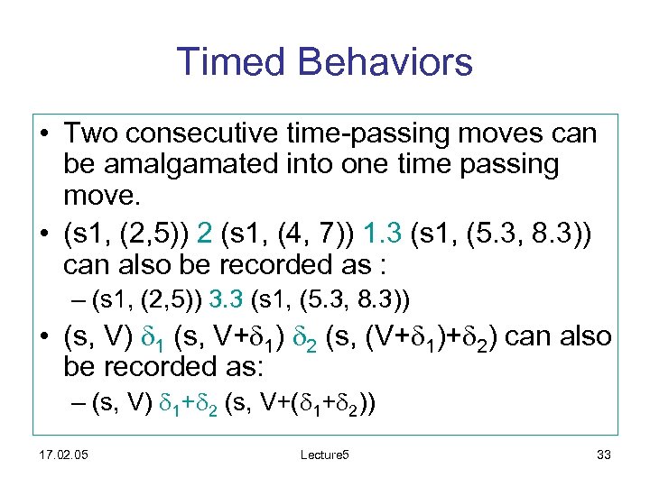Timed Behaviors • Two consecutive time-passing moves can be amalgamated into one time passing move. • (s 1, (2, 5)) 2 (s 1, (4, 7)) 1. 3 (s 1, (5. 3, 8. 3)) can also be recorded as : – (s 1, (2, 5)) 3. 3 (s 1, (5. 3, 8. 3)) • (s, V) 1 (s, V+ 1) 2 (s, (V+ 1)+ 2) can also be recorded as: – (s, V) 1+ 2 (s, V+( 1+ 2)) 17. 02. 05 Lecture 5 33

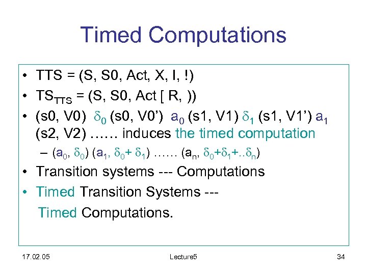Timed Computations • TTS = (S, S 0, Act, X, I, !) • TSTTS = (S, S 0, Act [ R, )) • (s 0, V 0) 0 (s 0, V 0’) a 0 (s 1, V 1) 1 (s 1, V 1’) a 1 (s 2, V 2) …… induces the timed computation – (a 0, 0) (a 1, 0+ 1) …… (an, 0+ 1+. . n) • Transition systems --- Computations • Timed Transition Systems --Timed Computations. 17. 02. 05 Lecture 5 34

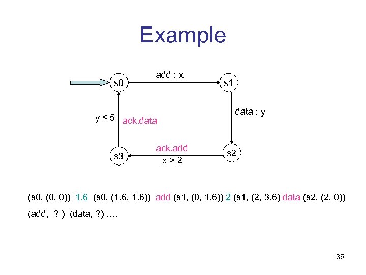Example s 0 add ; x y ≤ 5 ack. data s 3 ack. add x>2 s 1 data ; y s 2 (s 0, (0, 0)) 1. 6 (s 0, (1. 6, 1. 6)) add (s 1, (0, 1. 6)) 2 (s 1, (2, 3. 6) data (s 2, (2, 0)) (add, ? ) (data, ? ) …. 35

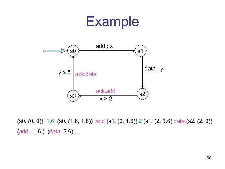Example s 0 add ; x y ≤ 5 ack. data s 3 ack. add x>2 s 1 data ; y s 2 (s 0, (0, 0)) 1. 6 (s 0, (1. 6, 1. 6)) add (s 1, (0, 1. 6)) 2 (s 1, (2, 3. 6) data (s 2, (2, 0)) (add, 1. 6 ) (data, 3. 6) …. 36

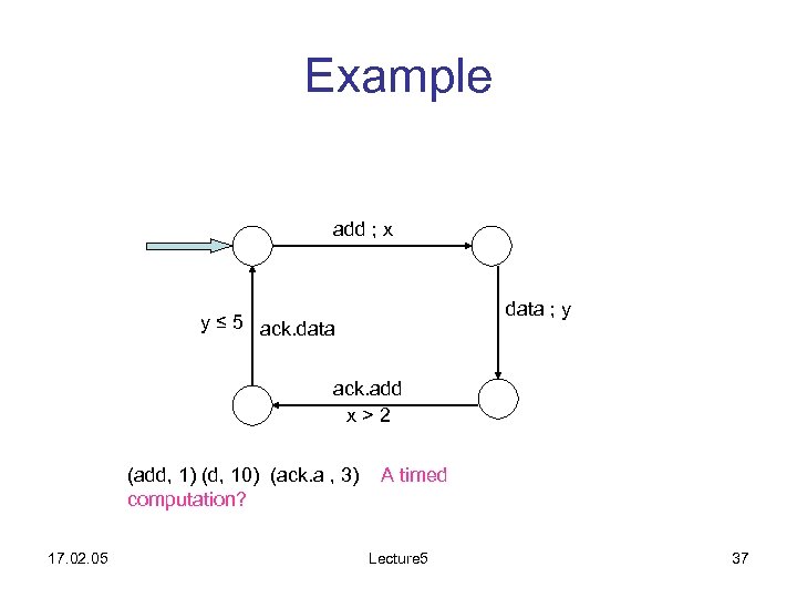Example add ; x data ; y y ≤ 5 ack. data ack. add x>2 (add, 1) (d, 10) (ack. a , 3) computation? 17. 02. 05 A timed Lecture 5 37

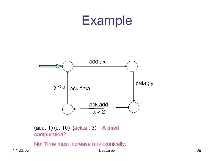Example add ; x data ; y y ≤ 5 ack. data ack. add x>2 (add, 1) (d, 10) (ack. a , 3) computation? A tmed No! Time must increase monotonically. 17. 02. 05 Lecture 5 38

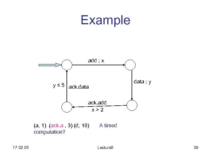Example add ; x data ; y y ≤ 5 ack. data ack. add x>2 (a, 1) (ack. a , 3) (d, 10) computation? 17. 02. 05 A timed Lecture 5 39

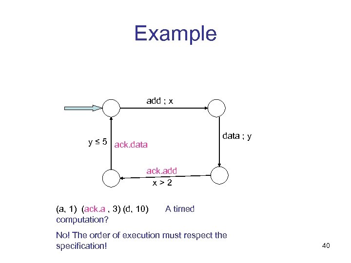Example add ; x data ; y y ≤ 5 ack. data ack. add x>2 (a, 1) (ack. a , 3) (d, 10) computation? A timed No! The order of execution must respect the specification! 40

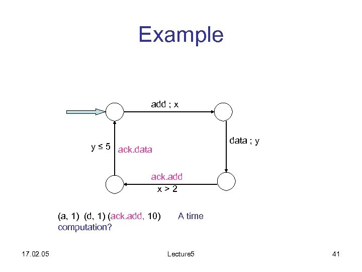Example add ; x data ; y y ≤ 5 ack. data ack. add x>2 (a, 1) (d, 1) (ack. add, 10) computation? 17. 02. 05 A time Lecture 5 41

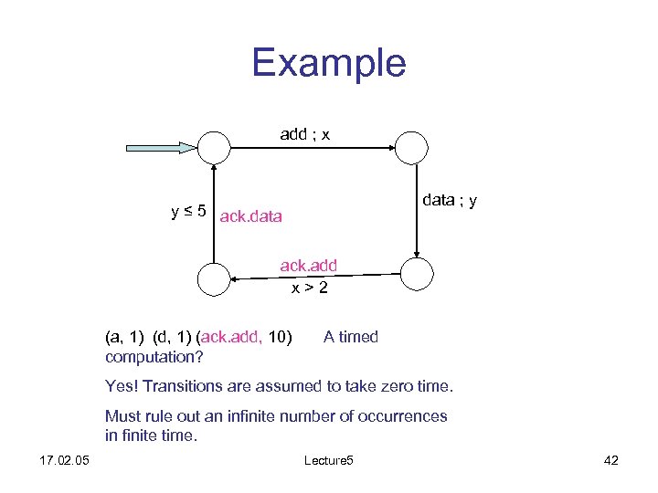Example add ; x data ; y y ≤ 5 ack. data ack. add x>2 (a, 1) (d, 1) (ack. add, 10) computation? A timed Yes! Transitions are assumed to take zero time. Must rule out an infinite number of occurrences in finite time. 17. 02. 05 Lecture 5 42

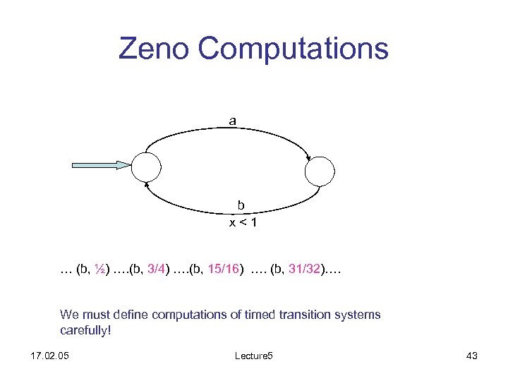Zeno Computations a b x<1 … (b, ½) …. (b, 3/4) …. (b, 15/16) …. (b, 31/32)…. We must define computations of timed transition systems carefully! 17. 02. 05 Lecture 5 43

Parallel Composition • TTS = TTS_1 || TTS_2 || …… || TTS_n • Same principle as before: – Do common actions together – Take union of clock variables. – Take conjunction of the guards! 17. 02. 05 Lecture 5 44

Reachability of Control States • For a finite TS it is trivial to decide whether s is reachable in TS. • For finite TTS, whether s is reachable in TTS is not easy to decide because TSTTS is an infinite object! • But this can be done and this verification process can be automated. • More involved (liveness) properties can also be verified effectively but not always efficiently. 17. 02. 05 Lecture 5 45

An introduction to UPPAAL CS 5272 - 18 Feb 2005 46

What is UPPAAL? • A toolbox for modeling, simulation and verification of real-time systems – Developed jointly by Uppsala University and Aalborg University – Often used for real-time controllers, communication protocols, etc. • Consists of 3 main parts – a system description – a simulator – a verifier 17. 02. 05 Lecture 5 47

System Description 17. 02. 05 Lecture 5 48

System Description • A system in UPPAAL: a set of concurrent processes • A process: a timed-automaton with: – Clocks and data variables – data variables: int, bool, array of int/bool • Scopes: global or local (to a process) – Both clocks and data variables! – Guards (on transitions) and invariants (on locations) are conditions on data variables and clocks 17. 02. 05 Lecture 5 49

System Description • Synchronization actions are described using communication channels • Two processes communicate with each other via global data variables or synchronization on communication channels 17. 02. 05 Lecture 5 50

System Description • A system description in UPPAAL is composed of – – 17. 02. 05 Global declarations Process templates Process assignments A system definition Lecture 5 51

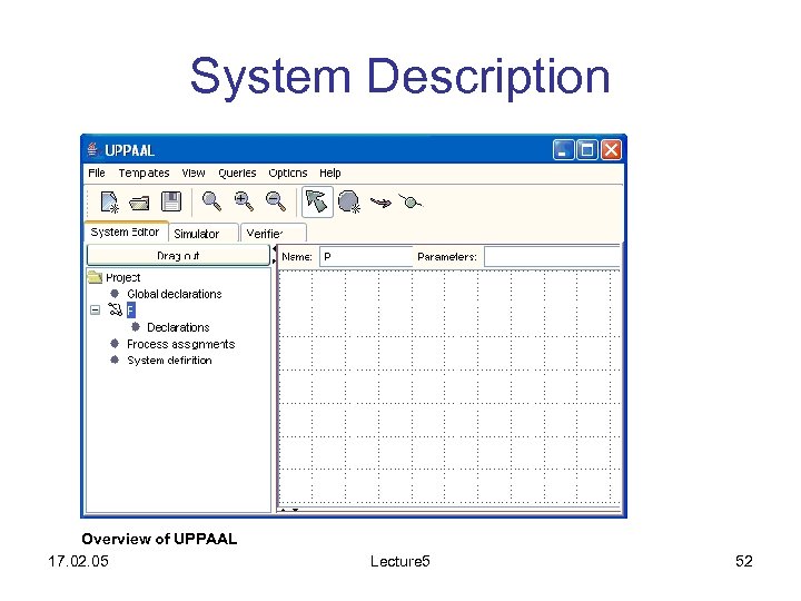System Description Overview of UPPAAL 17. 02. 05 Lecture 5 52

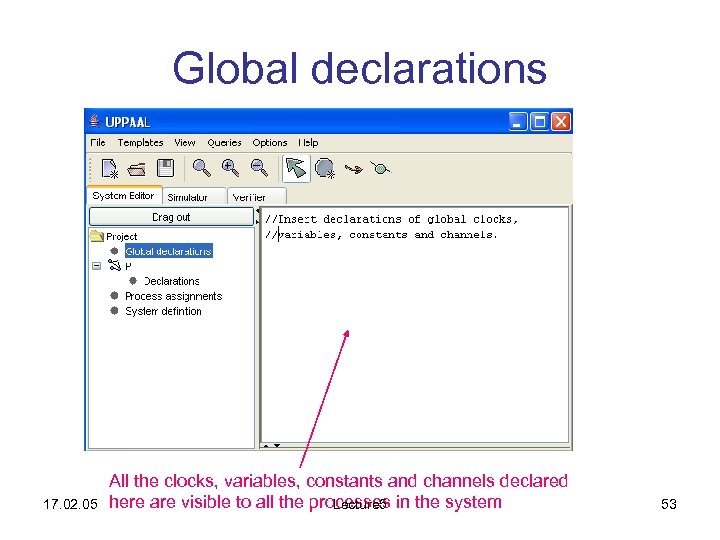Global declarations 17. 02. 05 All the clocks, variables, constants and channels declared here are visible to all the processes in the system Lecture 5 53

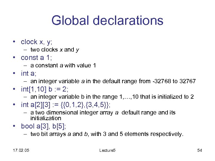Global declarations • clock x, y; – two clocks x and y • const a 1; – a constant a with value 1 • int a; – an integer variable a in the default range from -32768 to 32767 • int[1, 10] b : = 2; – an integer variable b in the range 1, …, 10 that is initialized to 2 • int a[2][3] : = {{0, 1, 2}, {3, 4, 5}}; – a two dimensional integer array a default range and its initialization • bool a[3], b[5]; – two bit arrays a and b, with 3 and 5 elements respectively. 17. 02. 05 Lecture 5 54

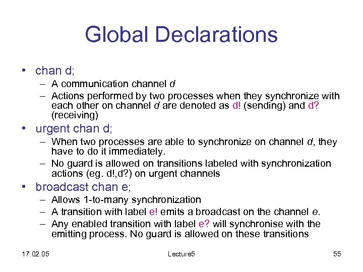Global Declarations • chan d; – A communication channel d – Actions performed by two processes when they synchronize with each other on channel d are denoted as d! (sending) and d? (receiving) • urgent chan d; – When two processes are able to synchronize on channel d, they have to do it immediately. – No guard is allowed on transitions labeled with synchronization actions (eg. d!, d? ) on urgent channels • broadcast chan e; – Allows 1 -to-many synchronization – A transition with label e! emits a broadcast on the channel e. – Any enabled transition with label e? will synchronise with the emitting process. No guard is allowed on these transitions 17. 02. 05 Lecture 5 55

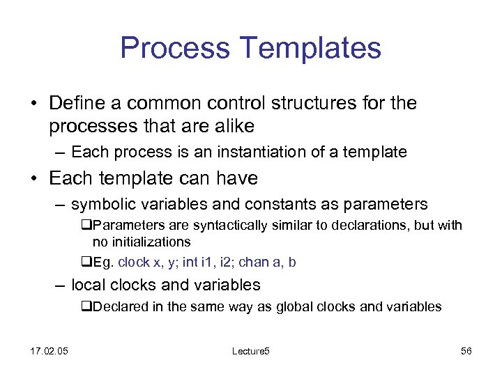Process Templates • Define a common control structures for the processes that are alike – Each process is an instantiation of a template • Each template can have – symbolic variables and constants as parameters q. Parameters are syntactically similar to declarations, but with no initializations q. Eg. clock x, y; int i 1, i 2; chan a, b – local clocks and variables q. Declared in the same way as global clocks and variables 17. 02. 05 Lecture 5 56

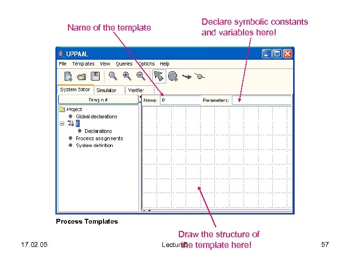Name of the template Declare symbolic constants and variables here! Process Templates 17. 02. 05 Draw the structure of Lecture 5 template here! the 57

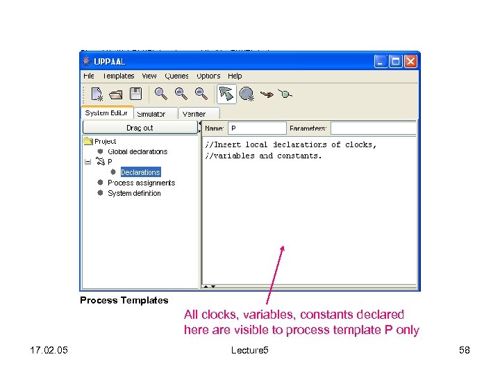Process Templates All clocks, variables, constants declared here are visible to process template P only 17. 02. 05 Lecture 5 58

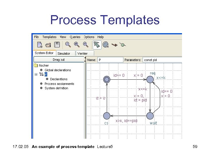Process Templates 17. 02. 05 An example of process template Lecture 5 59

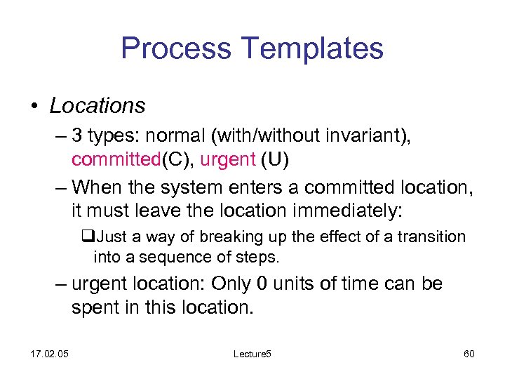Process Templates • Locations – 3 types: normal (with/without invariant), committed(C), urgent (U) – When the system enters a committed location, it must leave the location immediately: q. Just a way of breaking up the effect of a transition into a sequence of steps. – urgent location: Only 0 units of time can be spent in this location. 17. 02. 05 Lecture 5 60

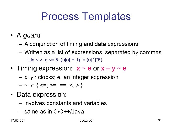Process Templates • A guard – A conjunction of timing and data expressions – Written as a list of expressions, separated by commas qx < y, x <= 5, (a[0] + 1) != (a[1]*5) • Timing expression: x ~ e or x – y ~ e – x, y : clocks; e: an integer expression – ~ { <=, >=, ==, <, > } • Data expression: – involves constants and variables – same as in C/C++/Java 17. 02. 05 Lecture 5 61

Process Templates • Invariants – Same as guards, with no lower bounds on clocks • Updates – A list of assignment expressions – Each assignment is of the form: x : = e or a : = e’ q. In x: = e, almost always e is 0. qx: a clock qa: a variable qe: an integer expression qe’: a data expression – Evaluated sequentially qa : = 1, b : = 2*a sets a to 1, b to 2. 17. 02. 05 Lecture 5 62

Process Assignments • Declare instances of process templates • Each assignment has the form P : = T(A); – P : a process name – T : a process template name – A : an argument list • Examples: – P : = Q(); q. Process P is an instance of template Q that has no parameter – S: =R(x, 1); q. Process S is an instance of template R that has two parameters - a clock and a constant 17. 02. 05 Lecture 5 63

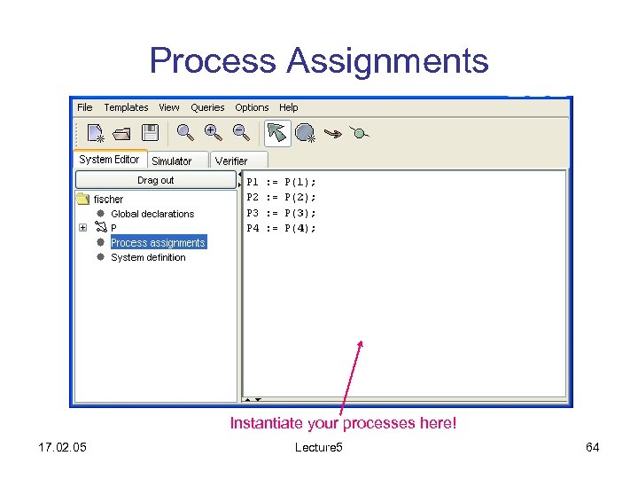Process Assignments Instantiate your processes here! 17. 02. 05 Lecture 5 64

System Definition • Declare the set of processes in the system • Eg. system P, Q; – A system consists of two processes P and Q • Each process in the system must be either – a process that appears on the left-hand-side of a process assignment, or – a template with no parameter 17. 02. 05 Lecture 5 65

Simulator 17. 02. 05 Lecture 5 66

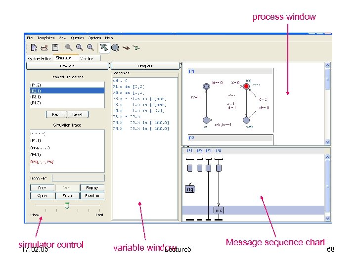
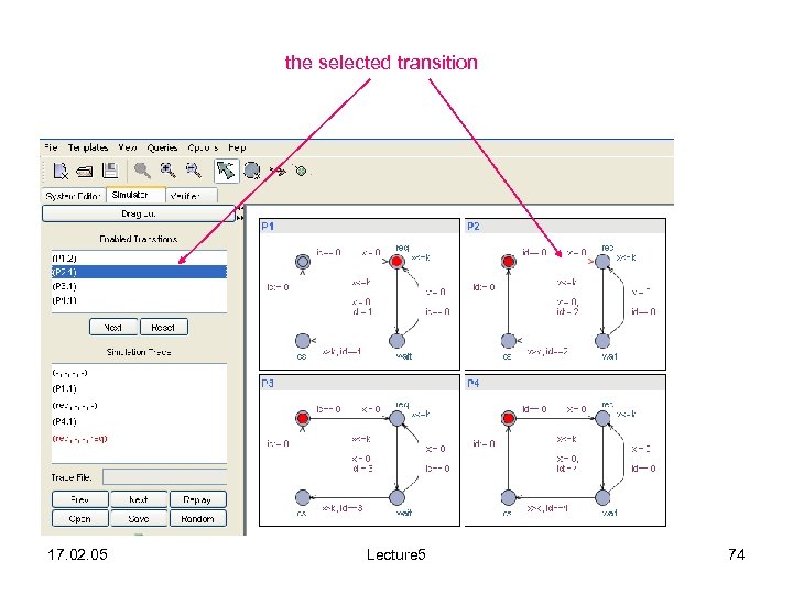
Simulator • A validation tool that – allows users to interact and observe the behavior of the system during execution – visualise executions (i. e. symbolic traces) generated by the verifier • Interface: divided into 4 sub-windows – – 17. 02. 05 Simulation control Variable window Process window Message Sequence Chart Lecture 5 67

process window simulator control 17. 02. 05 variable window Lecture 5 Message sequence chart 68

Simulator Control • Used to control the simulation and to select the (symbolic) state or transition to be visualized – Upper part: for step-by-step simulation q. Displays all enabled transitions q. Enables users to select an enabled transition to be fired – Lower part: displays the generated trace q. A trace is an alternating sequence of location vectors and transitions. 17. 02. 05 Lecture 5 69

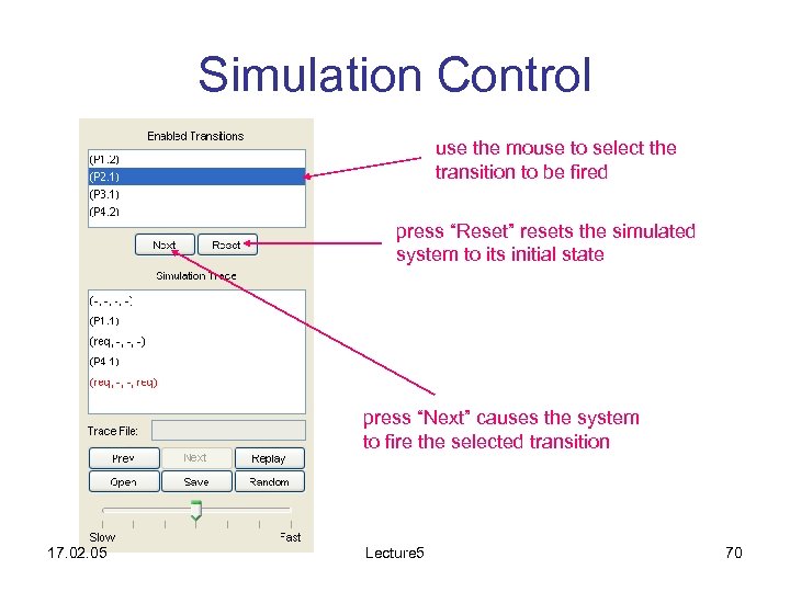Simulation Control use the mouse to select the transition to be fired press “Reset” resets the simulated system to its initial state press “Next” causes the system to fire the selected transition 17. 02. 05 Lecture 5 70

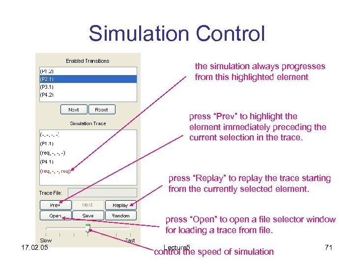Simulation Control the simulation always progresses from this highlighted element press “Prev” to highlight the element immediately preceding the current selection in the trace. press “Replay” to replay the trace starting from the currently selected element. press “Open” to open a file selector window for loading a trace from file. 17. 02. 05 Lecture 5 control the speed of simulation 71

Variable window • Displays the values of data and clocks in the current state or transition selected in the trace 17. 02. 05 Lecture 5 72

Process window • Displays the process instances of the system – The current location of each automaton is marked with a red token – The transitions currently selected in the simulation control panel are highlighted 17. 02. 05 Lecture 5 73

the selected transition 17. 02. 05 Lecture 5 74

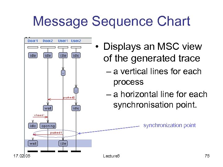Message Sequence Chart • Displays an MSC view of the generated trace – a vertical lines for each process – a horizontal line for each synchronisation point. synchronization point 17. 02. 05 Lecture 5 75

Verifier 17. 02. 05 Lecture 5 76

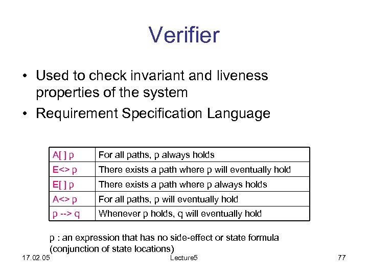Verifier • Used to check invariant and liveness properties of the system • Requirement Specification Language A[ ] p For all paths, p always holds E<> p There exists a path where p will eventually hold E[ ] p There exists a path where p always holds A<> p For all paths, p will eventually hold p --> q Whenever p holds, q will eventually hold p : an expression that has no side-effect or state formula (conjunction of state locations) 17. 02. 05 Lecture 5 77

Verifier • Examples • A[] not deadlock qtrue if the system is not deadlocked. – E<> p 1. cs and p 2. cs qtrue if the system can reach a state where both process p 1 and p 2 are in their locations cs. • A[ ] p 1. cs imply not p 2. cs qtrue if whenever process p 1 is in its location cs, the process is not in its location cs. 17. 02. 05 Lecture 5 78

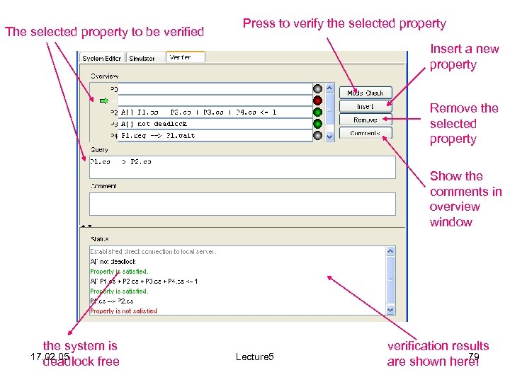The selected property to be verified Press to verify the selected property Insert a new property Remove the selected property Show the comments in overview window the system is 17. 02. 05 deadlock free Lecture 5 verification results 79 are shown here!