Time Varying Risk Aversion Luigi Guiso Einaudi

Time Varying Risk Aversion Luigi Guiso (Einaudi Institute for Economics & Finance- EIEF) Paola Sapienza (Northwestern University) Luigi Zingales (University of Chicago) Banca d’Italia, December 3 2015

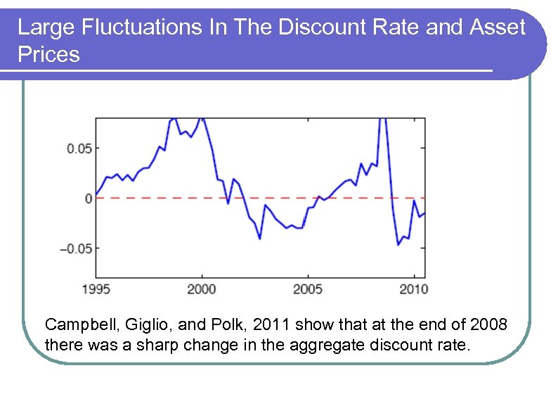Large Fluctuations In The Discount Rate and Asset Prices Campbell, Giglio, and Polk, 2011 show that at the end of 2008 there was a sharp change in the aggregate discount rate.

Where do they come from? l Fluctuations in the individual risk aversion l Shifts in the distribution of wealth that change the aggregate risk aversion l Changes in “sentiment”

What Explains Them? l If changes in individual risk aversion, what explains them? l Changes in wealth ? l l l Changes in preferences (curvature)? l l l Due to habit persistence ? Due to loss version? Why? At the center of the debate on rationality of markets At the center of the debate on fair value accounting

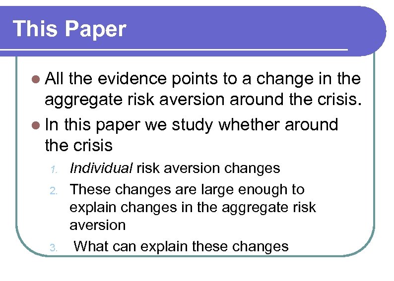This Paper l All the evidence points to a change in the aggregate risk aversion around the crisis. l In this paper we study whether around the crisis 1. 2. 3. Individual risk aversion changes These changes are large enough to explain changes in the aggregate risk aversion What can explain these changes

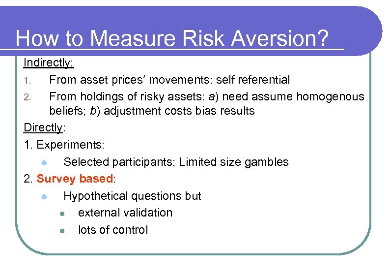How to Measure Risk Aversion? Indirectly: 1. From asset prices’ movements: self referential 2. From holdings of risky assets: a) need assume homogenous beliefs; b) adjustment costs bias results Directly: 1. Experiments: l Selected participants; Limited size gambles 2. Survey based: l Hypothetical questions but l external validation l lots of control

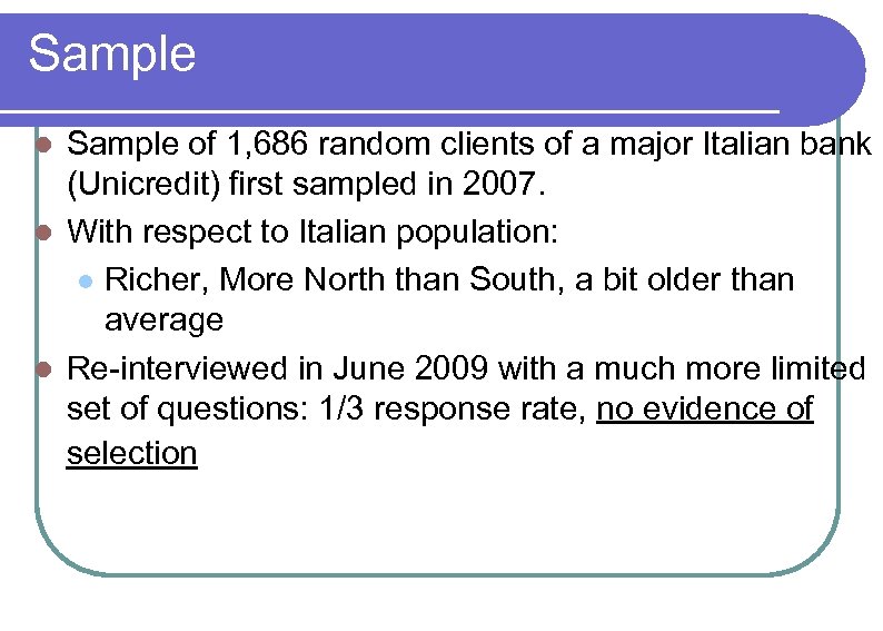Sample of 1, 686 random clients of a major Italian bank (Unicredit) first sampled in 2007. l With respect to Italian population: l Richer, More North than South, a bit older than average l Re-interviewed in June 2009 with a much more limited set of questions: 1/3 response rate, no evidence of selection l

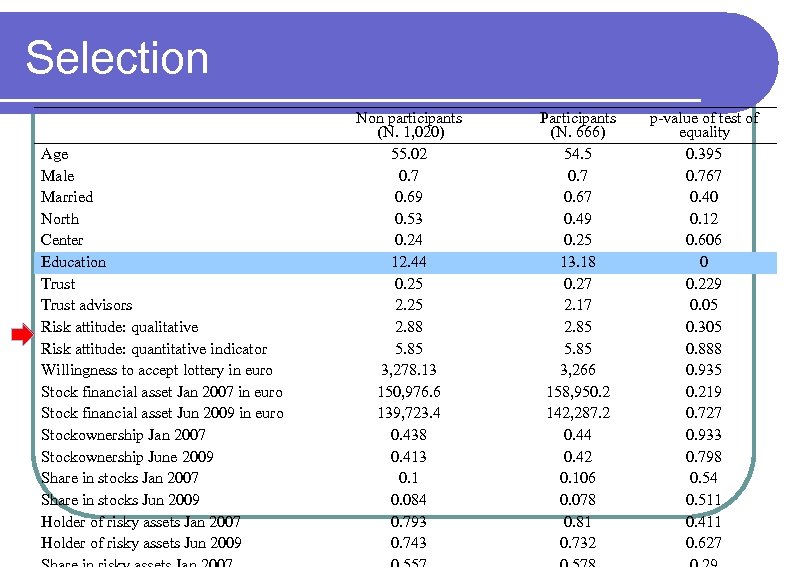Selection Age Male Married North Center Education Trust advisors Risk attitude: qualitative Risk attitude: quantitative indicator Willingness to accept lottery in euro Stock financial asset Jan 2007 in euro Stock financial asset Jun 2009 in euro Stockownership Jan 2007 Stockownership June 2009 Share in stocks Jan 2007 Share in stocks Jun 2009 Holder of risky assets Jan 2007 Holder of risky assets Jun 2009 Non participants (N. 1, 020) 55. 02 0. 7 0. 69 0. 53 0. 24 12. 44 0. 25 2. 88 5. 85 3, 278. 13 150, 976. 6 139, 723. 4 0. 438 0. 413 0. 1 0. 084 0. 793 0. 743 Participants (N. 666) 54. 5 0. 7 0. 67 0. 49 0. 25 13. 18 0. 27 2. 17 2. 85 5. 85 3, 266 158, 950. 2 142, 287. 2 0. 44 0. 42 0. 106 0. 078 0. 81 0. 732 p-value of test of equality 0. 395 0. 767 0. 40 0. 12 0. 606 0 0. 229 0. 05 0. 305 0. 888 0. 935 0. 219 0. 727 0. 933 0. 798 0. 54 0. 511 0. 411 0. 627

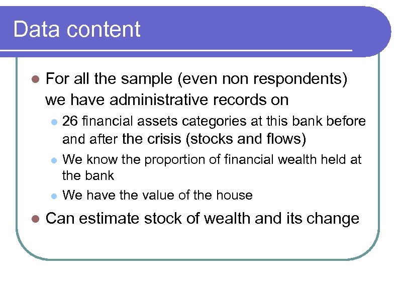Data content l For all the sample (even non respondents) we have administrative records on l l 26 financial assets categories at this bank before and after the crisis (stocks and flows) We know the proportion of financial wealth held at the bank We have the value of the house Can estimate stock of wealth and its change

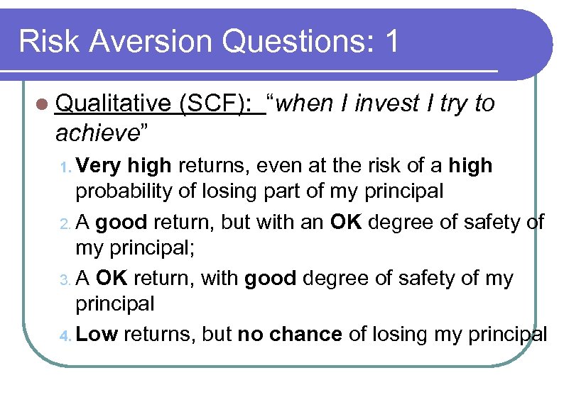Risk Aversion Questions: 1 l Qualitative (SCF): “when I invest I try to achieve” 1. Very high returns, even at the risk of a high probability of losing part of my principal 2. A good return, but with an OK degree of safety of my principal; 3. A OK return, with good degree of safety of my principal 4. Low returns, but no chance of losing my principal

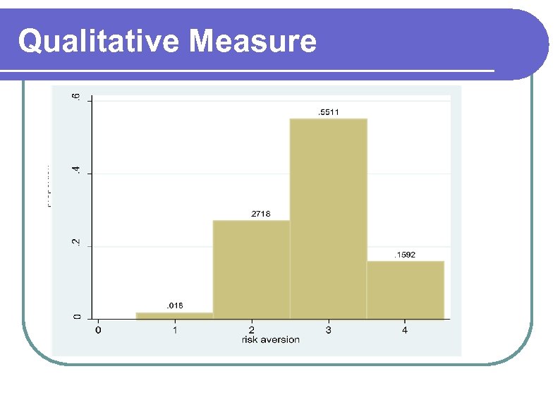Qualitative Measure

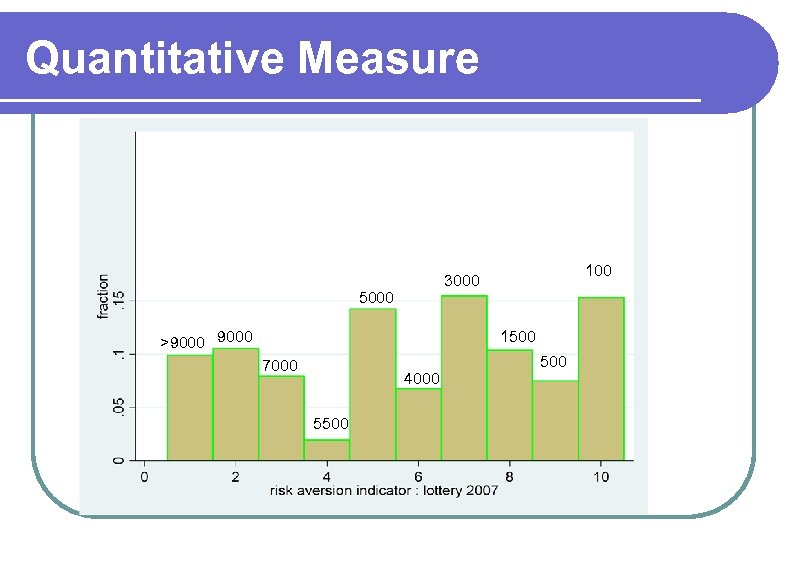
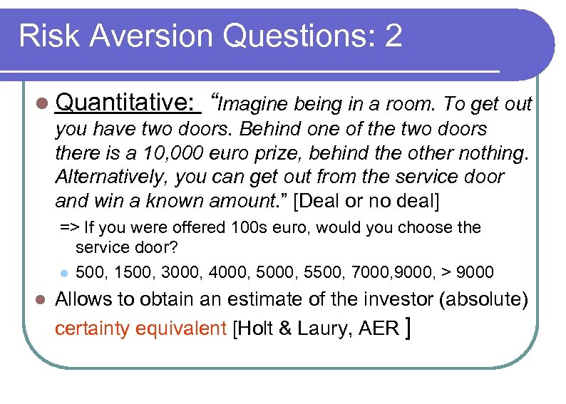Risk Aversion Questions: 2 l Quantitative: “Imagine being in a room. To get out you have two doors. Behind one of the two doors there is a 10, 000 euro prize, behind the other nothing. Alternatively, you can get out from the service door and win a known amount. ” [Deal or no deal] => If you were offered 100 s euro, would you choose the service door? l 500, 1500, 3000, 4000, 5500, 7000, 9000, > 9000 l Allows to obtain an estimate of the investor (absolute) certainty equivalent [Holt & Laury, AER ]

Quantitative Measure 100 3000 5000 >9000 1500 7000 4000 5500

Self Assessment l After the financial crisis, in your investment choices you are: 0: More or less like before 1: More cautious 2: Much more cautious

Outline 1. 2. 3. 4. 5. 6. 7. Are these measures just noise? Did they change enough? Why did they change? An hypothesis An experiment Conclusions

1 Are These Measures Just Noise?

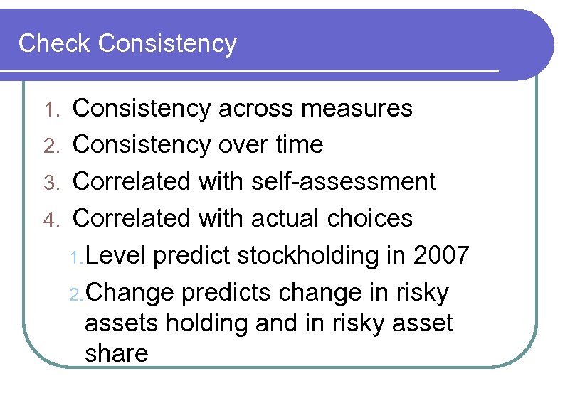Check Consistency across measures 2. Consistency over time 3. Correlated with self-assessment 4. Correlated with actual choices 1. Level predict stockholding in 2007 2. Change predicts change in risky assets holding and in risky asset share 1.

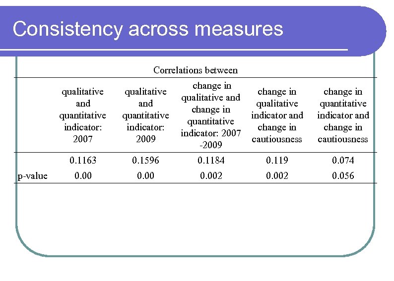Consistency across measures Correlations between qualitative and quantitative indicator: 2009 change in qualitative and change in quantitative indicator: 2007 -2009 change in qualitative indicator and change in cautiousness change in quantitative indicator and change in cautiousness 0. 1163 p-value qualitative and quantitative indicator: 2007 0. 1596 0. 1184 0. 119 0. 074 0. 002 0. 056

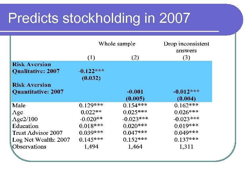Predicts stockholding in 2007

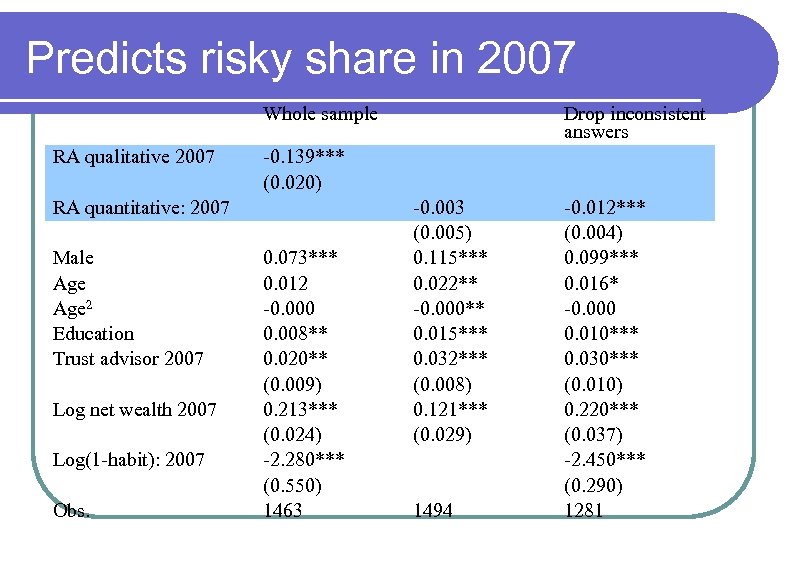Predicts risky share in 2007 Whole sample RA qualitative 2007 -0. 139*** (0. 020) RA quantitative: 2007 Male Age 2 Education Trust advisor 2007 Log net wealth 2007 Log(1 -habit): 2007 Obs. Drop inconsistent answers 0. 073*** 0. 012 -0. 000 0. 008** 0. 020** (0. 009) 0. 213*** (0. 024) -2. 280*** (0. 550) 1463 -0. 003 (0. 005) 0. 115*** 0. 022** -0. 000** 0. 015*** 0. 032*** (0. 008) 0. 121*** (0. 029) 1494 -0. 012*** (0. 004) 0. 099*** 0. 016* -0. 000 0. 010*** 0. 030*** (0. 010) 0. 220*** (0. 037) -2. 450*** (0. 290) 1281

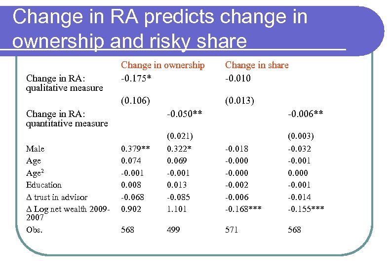Change in RA predicts change in ownership and risky share Change in share -0. 010 (0. 106) Change in RA: qualitative measure Change in ownership -0. 175* (0. 013) Change in RA: quantitative measure Male Age 2 Education Δ trust in advisor Δ Log net wealth 20092007 Obs. -0. 050** -0. 006** 0. 379** 0. 074 -0. 001 0. 008 -0. 068 0. 902 (0. 021) 0. 322* 0. 069 -0. 001 0. 013 -0. 085 1. 101 -0. 018 -0. 000 -0. 002 -0. 006 -0. 168*** (0. 003) -0. 032 -0. 001 0. 000 -0. 001 -0. 014 -0. 155*** 568 499 571 568

TVRA 2 Did These Measures Change?

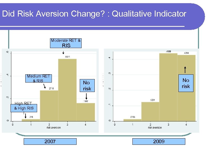Did Risk Aversion Change? : Qualitative Indicator Moderate RET & RIS Medium RET & RIS No risk High RET & High RIS i 2007 2009

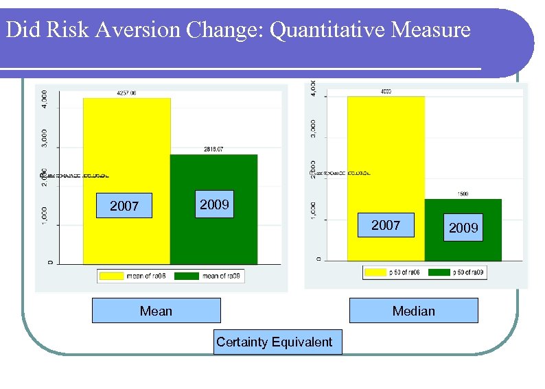Did Risk Aversion Change: Quantitative Measure 2009 2007 Mean Median Certainty Equivalent 2009

3 Did They Change Enough?

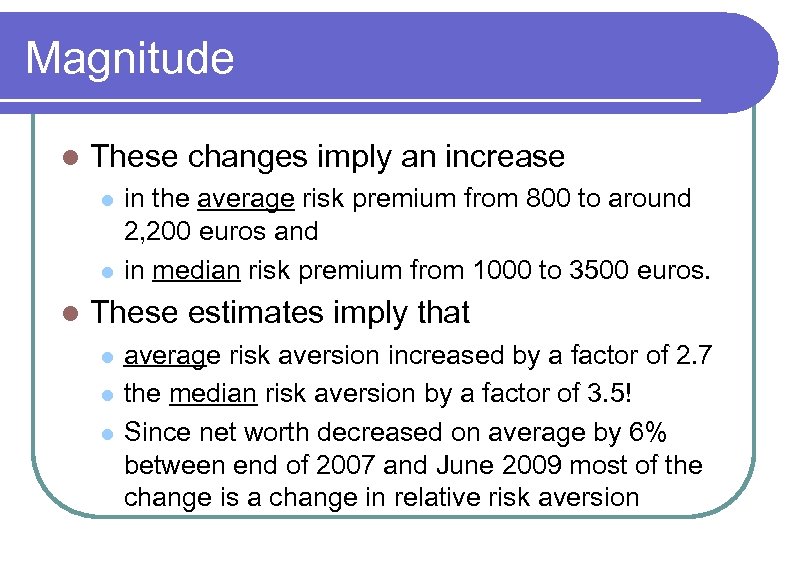Magnitude l These changes imply an increase l l l in the average risk premium from 800 to around 2, 200 euros and in median risk premium from 1000 to 3500 euros. These estimates imply that l l l average risk aversion increased by a factor of 2. 7 the median risk aversion by a factor of 3. 5! Since net worth decreased on average by 6% between end of 2007 and June 2009 most of the change is a change in relative risk aversion

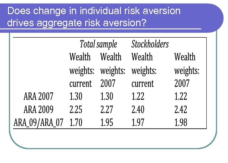Does change in individual risk aversion drives aggregate risk aversion?

4 What Does Explain These Changes?

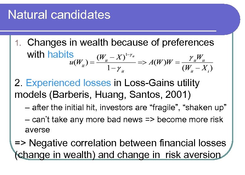Natural candidates 1. Changes in wealth because of preferences with habits 2. Experienced losses in Loss-Gains utility models (Barberis, Huang, Santos, 2001) – after the initial hit, investors are “fragile”, “shaken up” – can’t take any more bad news => become more risk averse => Negative correlation between financial losses (change in wealth) and change in risk aversion

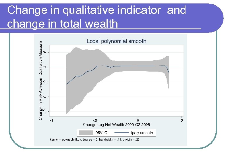
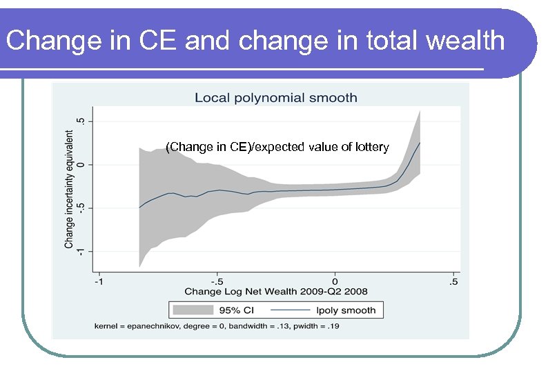
Evidence: non parametric l Estimate non parametric relation between change in risk aversion and financial losses during the crisis l Financial loss: l Proportional loss in financial portfolio between September 2008 (pre-Lehman) and February 2009 (bottom of stock market)

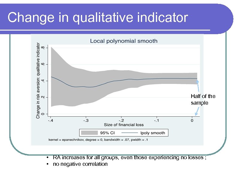Change in qualitative indicator Half of the sample • RA increases for all groups, even those experiencing no losses ; • no negative correlation

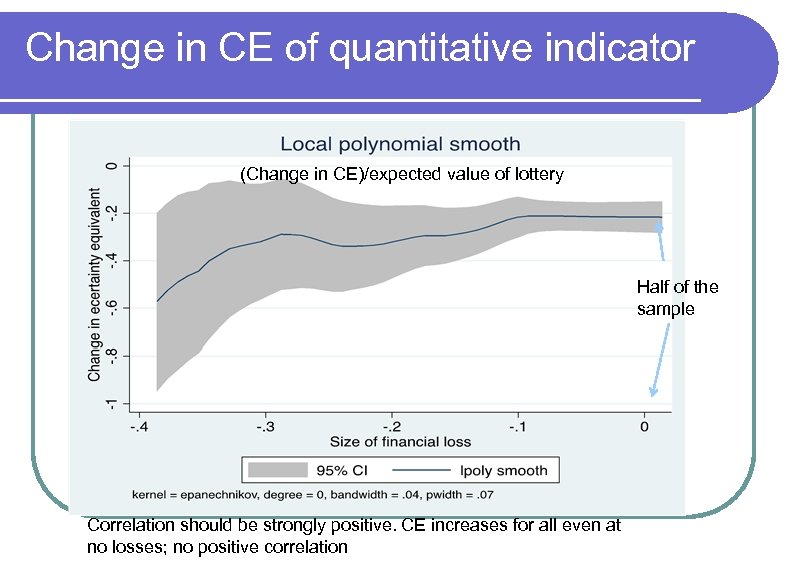Change in CE of quantitative indicator (Change in CE)/expected value of lottery Half of the sample Correlation should be strongly positive. CE increases for all even at no losses; no positive correlation

Change in qualitative indicator and change in total wealth

Change in CE and change in total wealth (Change in CE)/expected value of lottery

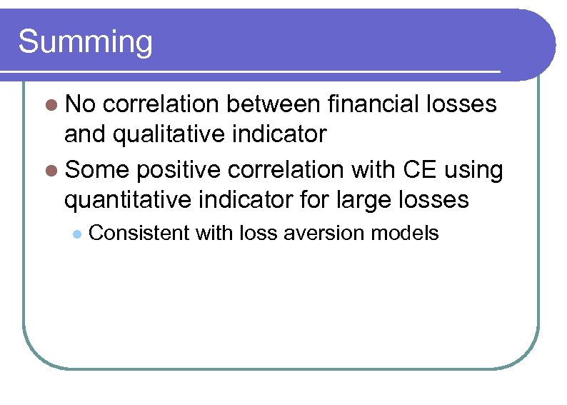Summing l No correlation between financial losses and qualitative indicator l Some positive correlation with CE using quantitative indicator for large losses l Consistent with loss aversion models

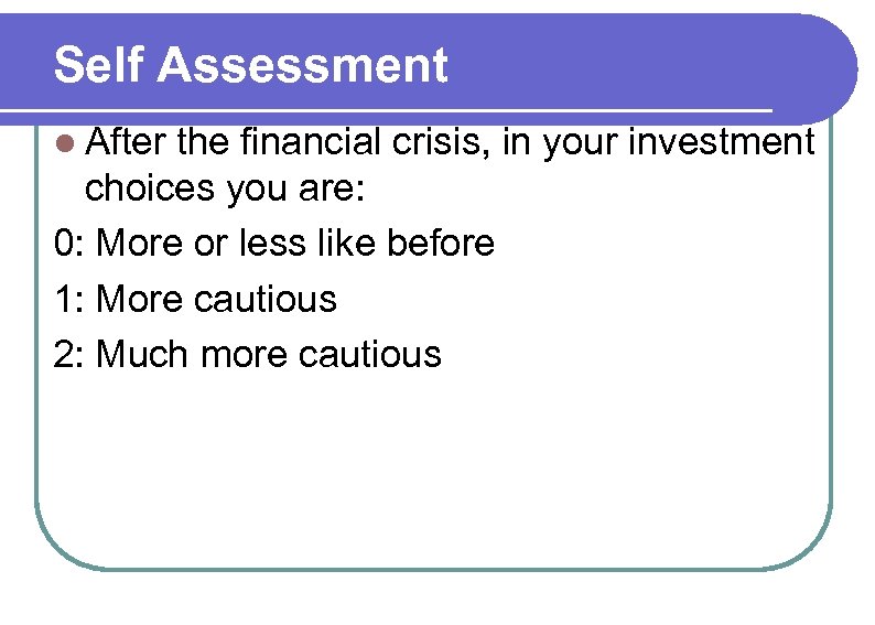
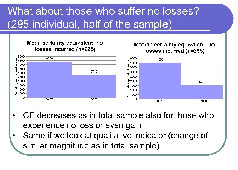What about those who suffer no losses? (295 individual, half of the sample) 5000 4500 4000 3500 3000 2500 2000 1500 1000 500 0 4350 2740 2007 2009 Median certainty equivalent: no losses incurred (n=295) Certainty equivalent: mean Mean certainty equivalent: no losses incurred (n=295) 4500 4000 3500 3000 2500 2000 1500 1000 500 0 2007 2009 • CE decreases as in total sample also for those who experience no loss or even gain • Same if we look at qualitative indicator (change of similar magnitude as in total sample)

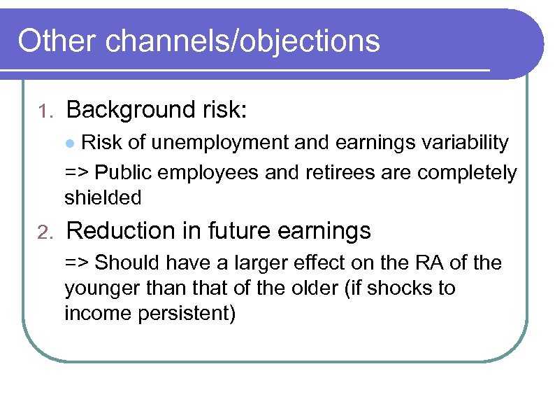Other channels/objections 1. Background risk: Risk of unemployment and earnings variability => Public employees and retirees are completely shielded l 2. Reduction in future earnings => Should have a larger effect on the RA of the younger than that of the older (if shocks to income persistent)

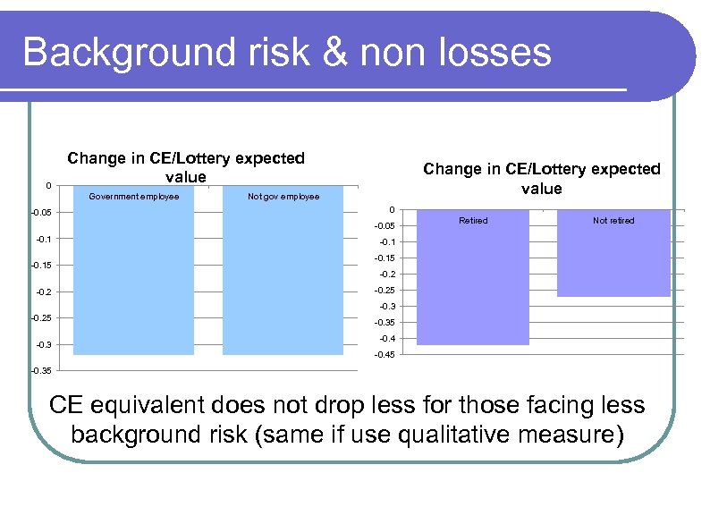Background risk & non losses 0 Change in CE/Lottery expected value Government employee -0. 05 Change in CE/Lottery expected value Not gov employee 0 -0. 05 -0. 15 -0. 2 Retired Not retired -0. 15 -0. 25 -0. 35 -0. 45 -0. 35 CE equivalent does not drop less for those facing less background risk (same if use qualitative measure)

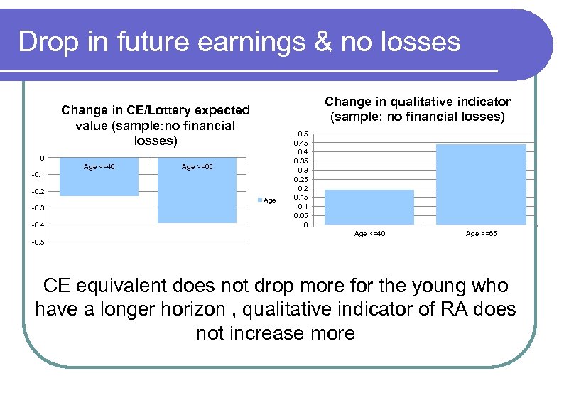Drop in future earnings & no losses Change in qualitative indicator (sample: no financial losses) Change in CE/Lottery expected value (sample: no financial losses) 0 Age <=40 Age >=65 -0. 1 -0. 2 Age -0. 3 -0. 4 0. 5 0. 4 0. 35 0. 3 0. 25 0. 2 0. 15 0. 1 0. 05 0 Age <=40 Age >=65 -0. 5 CE equivalent does not drop more for the young who have a longer horizon , qualitative indicator of RA does not increase more

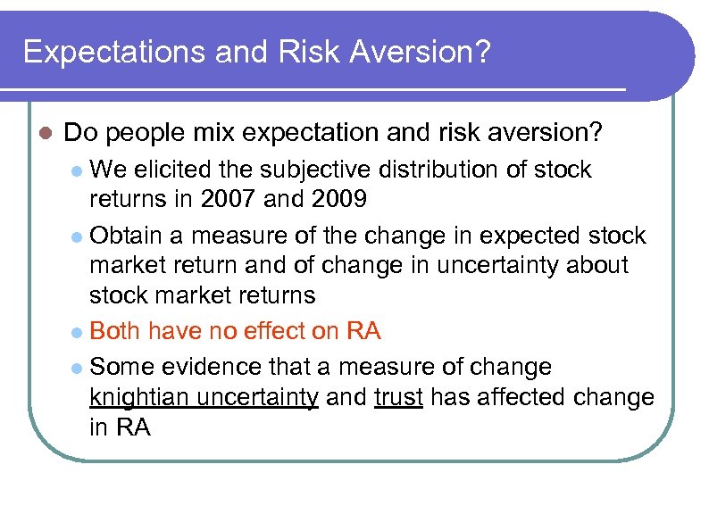Expectations and Risk Aversion? l Do people mix expectation and risk aversion? We elicited the subjective distribution of stock returns in 2007 and 2009 l Obtain a measure of the change in expected stock market return and of change in uncertainty about stock market returns l Both have no effect on RA l Some evidence that a measure of change knightian uncertainty and trust has affected change in RA l

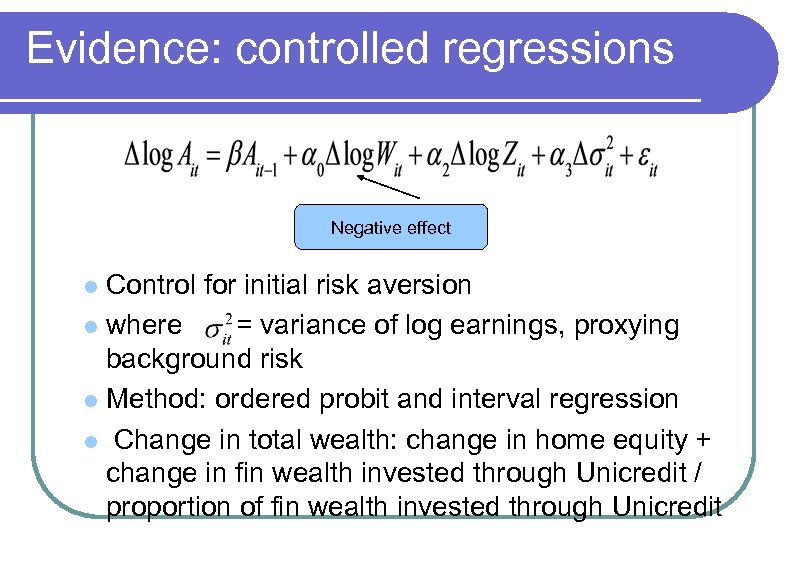
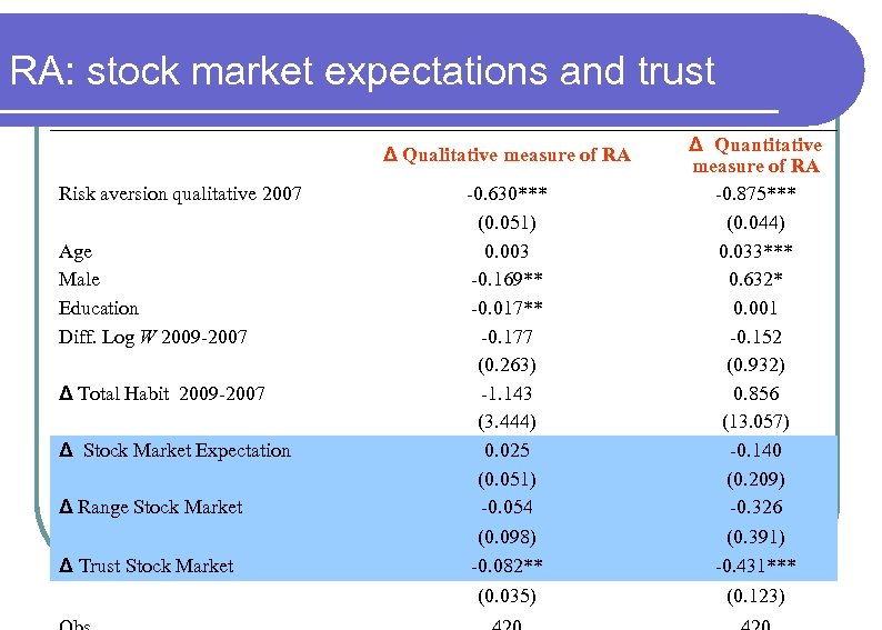RA: stock market expectations and trust Risk aversion qualitative 2007 Age Male Education Diff. Log W 2009 -2007 Δ Total Habit 2009 -2007 Δ Stock Market Expectation Δ Range Stock Market Δ Trust Stock Market Δ Qualitative measure of RA -0. 630*** (0. 051) 0. 003 -0. 169** -0. 017** -0. 177 (0. 263) -1. 143 (3. 444) 0. 025 (0. 051) -0. 054 (0. 098) -0. 082** (0. 035) Δ Quantitative measure of RA -0. 875*** (0. 044) 0. 033*** 0. 632* 0. 001 -0. 152 (0. 932) 0. 856 (13. 057) -0. 140 (0. 209) -0. 326 (0. 391) -0. 431*** (0. 123)

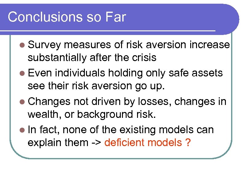Conclusions so Far l Survey measures of risk aversion increase substantially after the crisis l Even individuals holding only safe assets see their risk aversion go up. l Changes not driven by losses, changes in wealth, or background risk. l In fact, none of the existing models can explain them -> deficient models ?

5 An Hypothesis

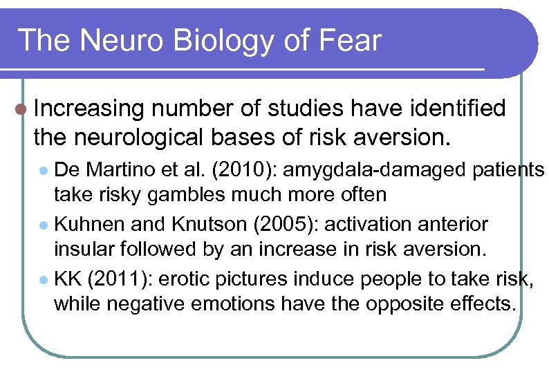The Neuro Biology of Fear l Increasing number of studies have identified the neurological bases of risk aversion. De Martino et al. (2010): amygdala-damaged patients take risky gambles much more often l Kuhnen and Knutson (2005): activation anterior insular followed by an increase in risk aversion. l KK (2011): erotic pictures induce people to take risk, while negative emotions have the opposite effects. l

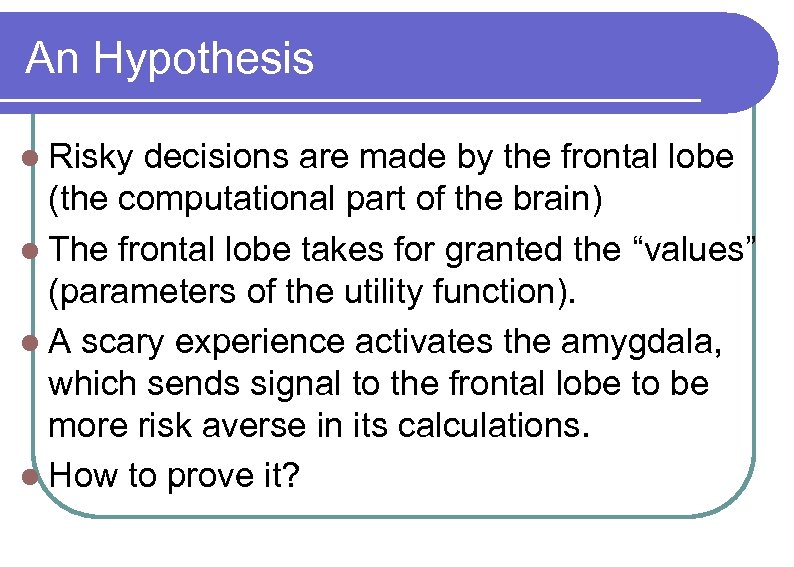An Hypothesis l Risky decisions are made by the frontal lobe (the computational part of the brain) l The frontal lobe takes for granted the “values” (parameters of the utility function). l A scary experience activates the amygdala, which sends signal to the frontal lobe to be more risk averse in its calculations. l How to prove it?

5 An Experiment

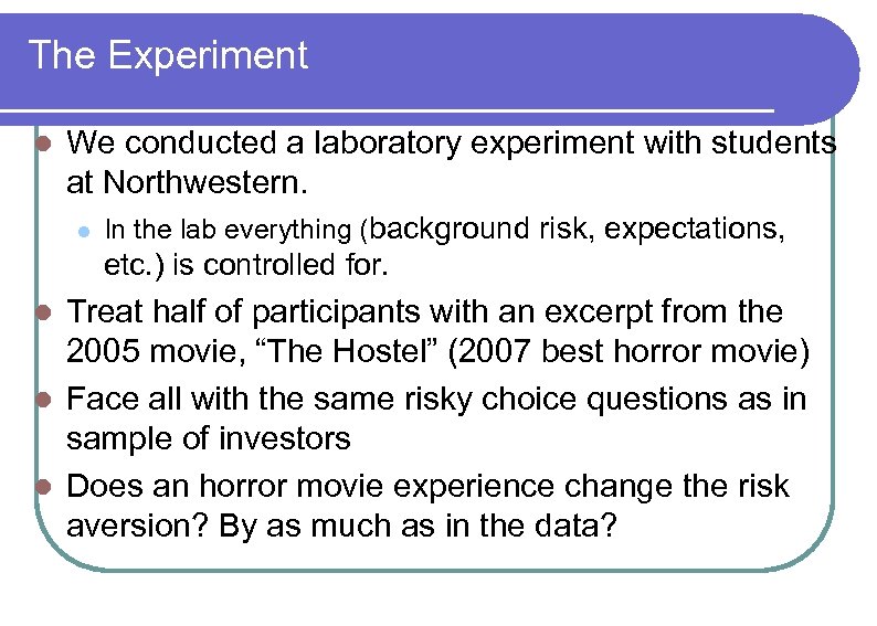The Experiment l We conducted a laboratory experiment with students at Northwestern. l In the lab everything (background risk, expectations, etc. ) is controlled for. Treat half of participants with an excerpt from the 2005 movie, “The Hostel” (2007 best horror movie) l Face all with the same risky choice questions as in sample of investors l Does an horror movie experience change the risk aversion? By as much as in the data? l

HOSTEL

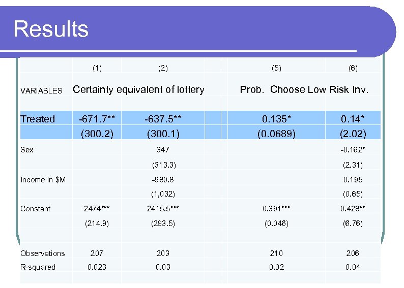Results VARIABLES Treated (1) (2) Certainty equivalent of lottery -671. 7** (300. 2) Sex (5) (6) Prob. Choose Low Risk Inv. -637. 5** (300. 1) 0. 135* (0. 0689) 0. 14* (2. 02) 347 (313. 3) 0. 195 (1, 032) Constant (2. 31) -980. 8 Income in $M -0. 162* (0. 65) R-squared 2415. 5*** 0. 391*** 0. 428** (214. 9) Observations 2474*** (293. 5) (0. 046) (6. 76) 207 203 210 206 0. 023 0. 02 0. 04

Heterogeneity Not everybody is scared the same. l Some people like horror movies. l Does the impact differ depending on how scared you were? l In half of the sample we asked people how much they liked horror movies on a scale from 0 to 100. l l Roughly a third do not like it at all

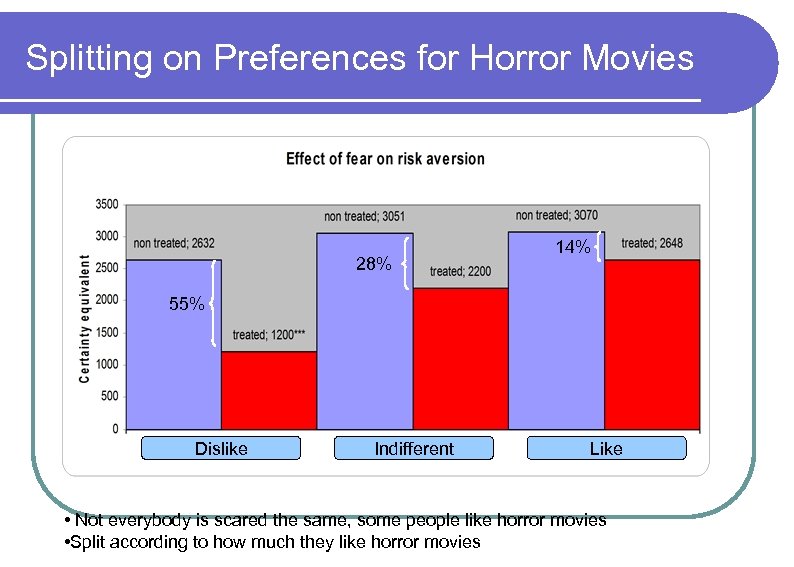Splitting on Preferences for Horror Movies 28% 14% 55% Dislike Indifferent Like • Not everybody is scared the same, some people like horror movies • Split according to how much they like horror movies

A Circular Argument? l Was an increase in risk aversion that caused the crash or vice versa? l Initial drop in expected cash flow -> fear -> -> increase in risk premium-> further drop l Our argument suggests that stock prices may overshoot movements in fundamentals (cash flow).

Conclusion l We showed that individual risk aversion increased a lot during the financial crisis: average risk aversion increased by a factor 2. 5 l median by a factor of 3. 5 l l These changes cannot be explained by standard models l They are consistent with a sudden increase in fear

Persistency? l Malmendier and Nagel (2011) find a cohort effect of depression-babies in the risk aversion measure of the SCF. l Unfortunately, our sample is unable to answer this question (even if we were to go back) because of the subsequent events in the eurozone that made the 2008 shock not an isolated incident.

Short and clearer version? Risk off “Why some people are more cautious with their finances than others”, The Economist, Jan 25 2014

Expectations l If you invest 10, 000 euro in a mutual fund that replicates the Italian stock market, in a year what is the 1. The minimum value of your investment 2. The maximum value of your investment 3. The probability that value greater than or equal to (Min+Max)/2 (uniform or triangular)

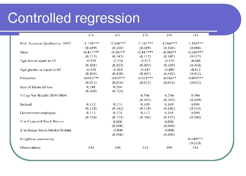
Evidence: controlled regressions Negative effect Control for initial risk aversion l where = variance of log earnings, proxying background risk l Method: ordered probit and interval regression l Change in total wealth: change in home equity + change in fin wealth invested through Unicredit / proportion of fin wealth invested through Unicredit l

Controlled regression

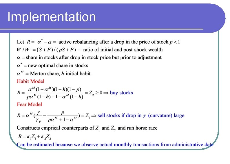
Noisy data or deficient models? l If RA measures just reflect noisy data they should have little predictive power on investors portfolio decisions l If have content, measured changes in risk aversion should be reflected in portfolio rebalancing

Implementation

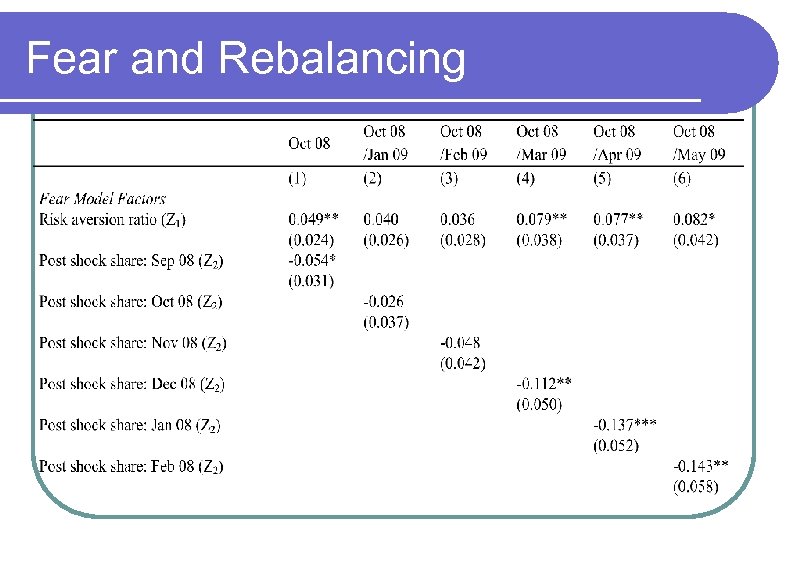
Rebalancing and risk aversion

6 Testing the Fear Hypothesis

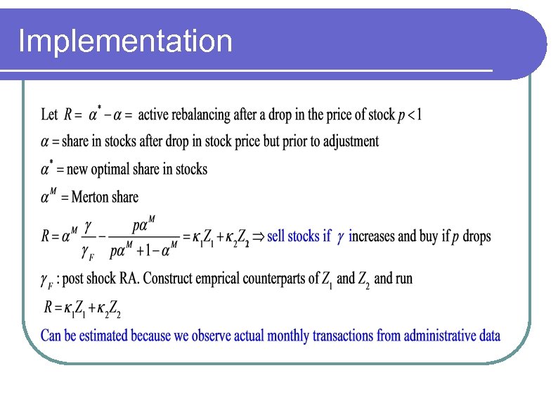
Discerning fear and habits l Experiment not directly connected to field data l Can we discern fear from habit in the data? l Models with habits and models with fear have different implications for active rebalancing after a shock to stock prices

Implementation

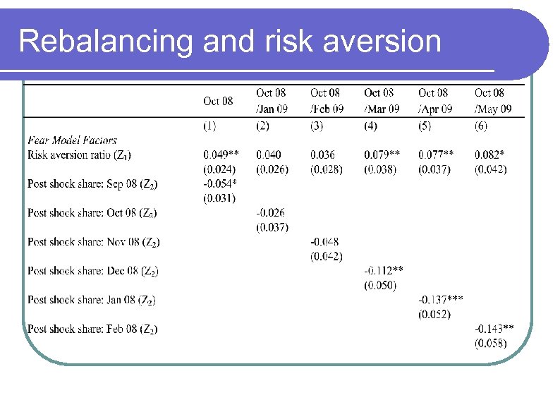
Fear and Rebalancing

Implications l The portfolio rebalancing we observe after the crisis is inconsistent with a model of habit persistence and consistent with a change in risk aversion driven by fear. l The fear-based model is also the only one able to account for the experimental evidence.

l Question designed to resemble a popular game (“Deal or no Deal”), analyzed by Bombardini and Trebbi (2010). l They find that in this game people exhibit a Von Neumann and Morgenstern utility function with a constant relative risk aversion close to 1.