Tier I Mathematical Methods of Click to edit

Tier I: Mathematical Methods of Click to edit Master title style Optimization Section 3: Nonlinear Programming

Introduction to Nonlinear Click to edit Master title style Programming • We already talked about a basic aspect of nonlinear programming (NLP) in the Introduction Chapter when we considered unconstrained optimization.

Introduction to Nonlinear Click to edit Master title style Programming • We optimized one-variable nonlinear functions using the 1 st and 2 nd derivatives. • We will use the same concept here extended to functions with more than one variable.

Multivariable Unconstrained Click to edit Master title style Optimization • For functions with one variable, we use the 1 st and 2 nd derivatives. • For functions with multiple variables, we use identical information that is the gradient and the Hessian. • The gradient is the first derivative with respect to all variables whereas the Hessian is the equivalent of the second derivative

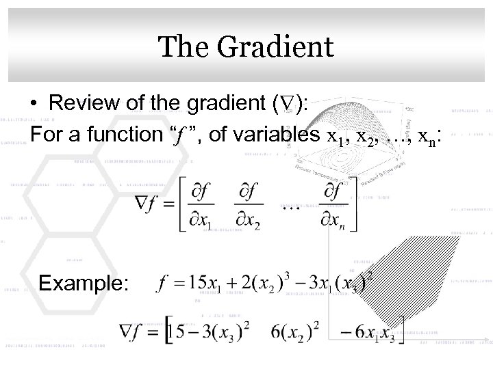Click to The Gradient style edit Master title • Review of the gradient ( ): For a function “f ”, of variables x 1, x 2, …, xn: Example:

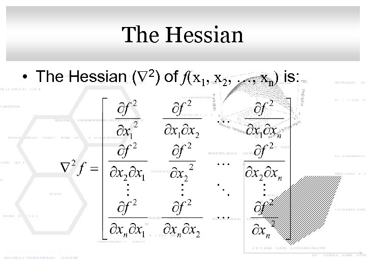Click to edit Master title style The Hessian • The Hessian ( 2) of f(x 1, x 2, …, xn) is:

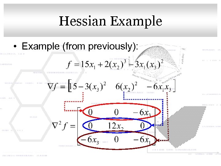Click to edit Master title style Hessian Example • Example (from previously):

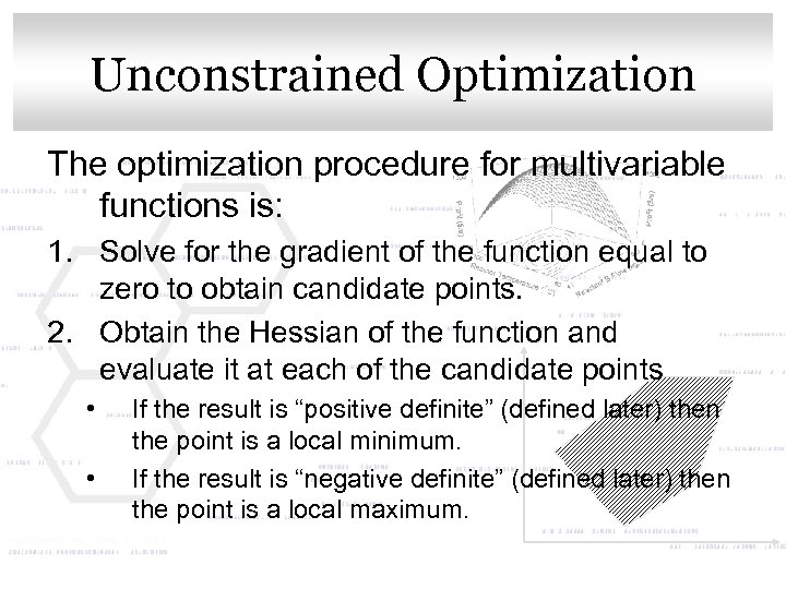Click to edit Master title style Unconstrained Optimization The optimization procedure for multivariable functions is: 1. Solve for the gradient of the function equal to zero to obtain candidate points. 2. Obtain the Hessian of the function and evaluate it at each of the candidate points • • If the result is “positive definite” (defined later) then the point is a local minimum. If the result is “negative definite” (defined later) then the point is a local maximum.

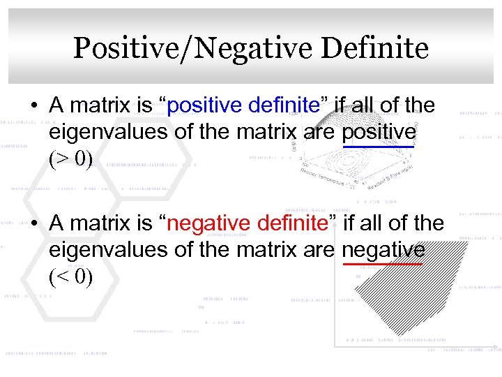Click to edit Master Definite Positive/Negative title style • A matrix is “positive definite” if all of the eigenvalues of the matrix are positive (> 0) • A matrix is “negative definite” if all of the eigenvalues of the matrix are negative (< 0)

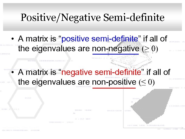Positive/Negative Semi-definite Click to edit Master title style • A matrix is “positive semi-definite” if all of the eigenvalues are non-negative (≥ 0) • A matrix is “negative semi-definite” if all of the eigenvalues are non-positive (≤ 0)

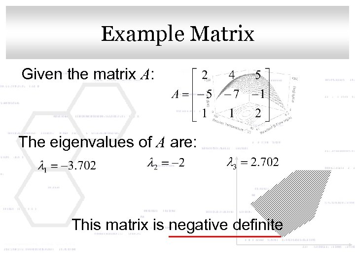Click to edit Master title style Example Matrix Given the matrix A: The eigenvalues of A are: This matrix is negative definite

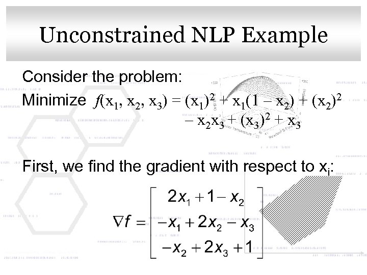Unconstrained NLP title style Click to edit Master Example Consider the problem: Minimize f(x 1, x 2, x 3) = (x 1)2 + x 1(1 – x 2) + (x 2)2 – x 2 x 3 + (x 3)2 + x 3 First, we find the gradient with respect to xi:

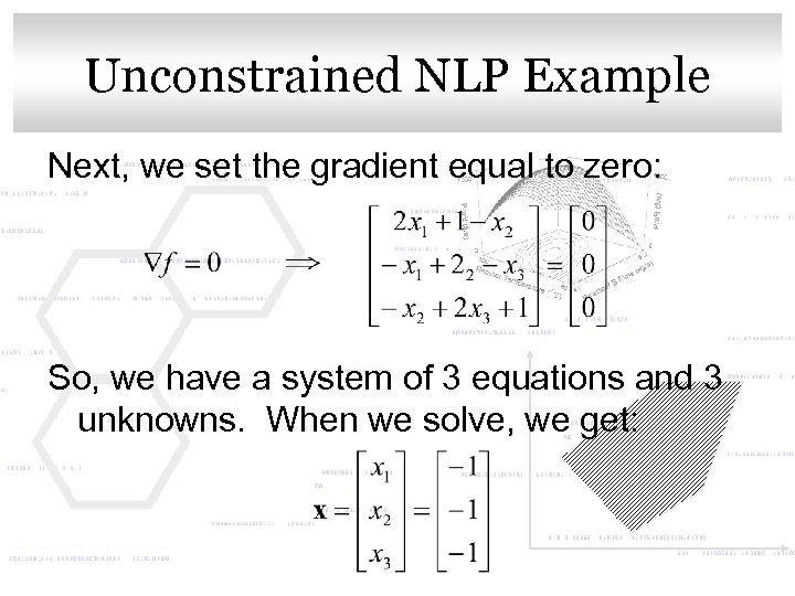Unconstrained NLP title style Click to edit Master Example Next, we set the gradient equal to zero: So, we have a system of 3 equations and 3 unknowns. When we solve, we get:

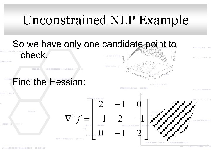Unconstrained NLP title style Click to edit Master Example So we have only one candidate point to check. Find the Hessian:

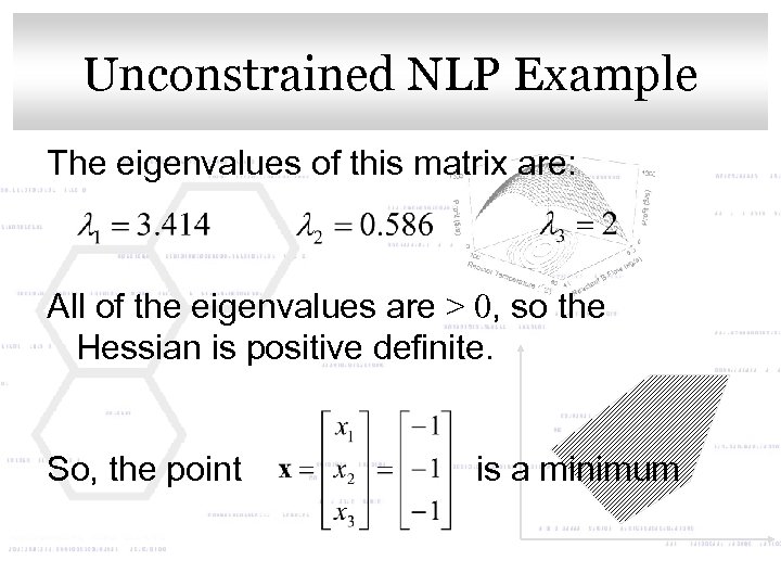Unconstrained NLP title style Click to edit Master Example The eigenvalues of this matrix are: All of the eigenvalues are > 0, so the Hessian is positive definite. So, the point is a minimum

Unconstrained NLP title style Click to edit Master Example Unlike in Linear Programming, unless we know the shape of the function being minimized or can determine whether it is convex, we cannot tell whether this point is the global minimum or if there are function values smaller than it.

Click. Method. Master title style to edit of Solution • In the previous example, when we set the gradient equal to zero, we had a system of 3 linear equations & 3 unknowns. • For other problems, these equations could be nonlinear. • Thus, the problem can become trying to solve a system of nonlinear equations, which can be very difficult.

Click. Method. Master title style to edit of Solution • To avoid this difficulty, NLP problems are usually solved numerically. • We will now look at examples of numerical methods used to find the optimum point for single-variable NLP problems. These and other methods may be found in any numerical methods reference.

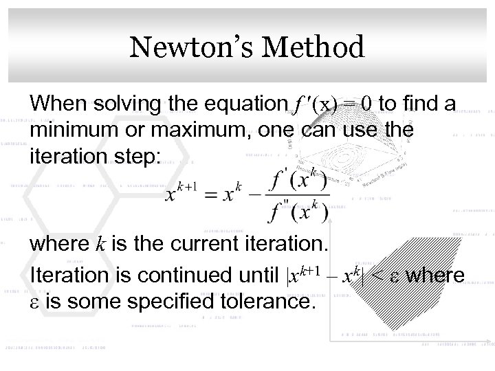Click to edit Master title style Newton’s Method When solving the equation f (x) = 0 to find a minimum or maximum, one can use the iteration step: where k is the current iteration. Iteration is continued until |xk+1 – xk| < e where e is some specified tolerance.

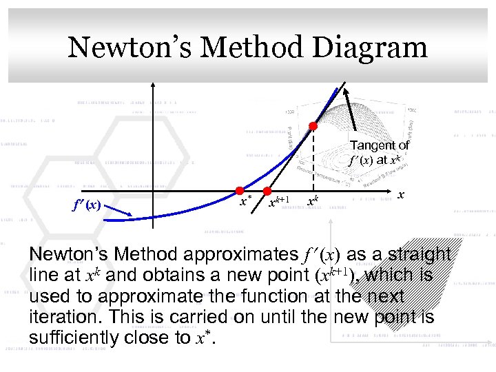Click to edit Master. Diagram Newton’s Method title style Tangent of f (x) at xk f (x) x* xk+1 xk x Newton’s Method approximates f (x) as a straight line at xk and obtains a new point (xk+1), which is used to approximate the function at the next iteration. This is carried on until the new point is sufficiently close to x*.

Click to edit Master title style Newton’s Method Comments • One must ensure that f (xk+1) < f (xk) for finding a minimum and f (xk+1) > f (xk) for finding a maximum. • Disadvantages: – Both the first and second derivatives must be calculated – The initial guess is very important – if it is not close enough to the solution, the method may not converge

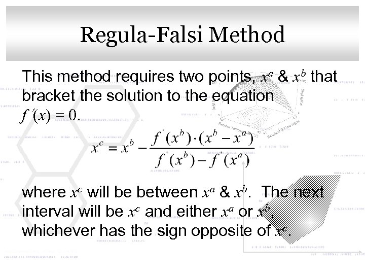Click to edit Master title style Regula-Falsi Method This method requires two points, xa & xb that bracket the solution to the equation f (x) = 0. where xc will be between xa & xb. The next interval will be xc and either xa or xb, whichever has the sign opposite of xc.

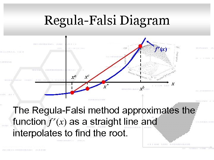Click to edit Master title style Regula-Falsi Diagram f (x) xa xc x* xb x The Regula-Falsi method approximates the function f (x) as a straight line and interpolates to find the root.

Click to edit Master title style Regula-Falsi Comments • This method requires initial knowledge of two points bounding the solution • However, it does not require the calculation of the second derivative • The Regula-Falsi Method requires slightly more iterations to converge than the Newton’s Method

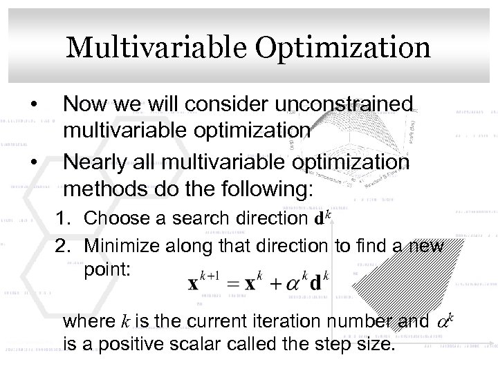Click to edit Master title style Multivariable Optimization • • Now we will consider unconstrained multivariable optimization Nearly all multivariable optimization methods do the following: 1. Choose a search direction dk 2. Minimize along that direction to find a new point: where k is the current iteration number and ak is a positive scalar called the step size.

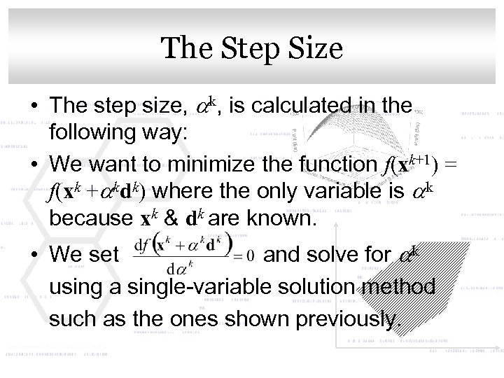Click to The Step Size style edit Master title • The step size, ak, is calculated in the following way: • We want to minimize the function f(xk+1) = f(xk +akdk) where the only variable is ak because xk & dk are known. • We set and solve for ak using a single-variable solution method such as the ones shown previously.

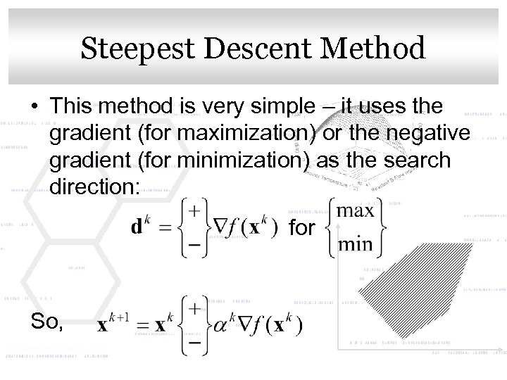Click to edit Master. Method Steepest Descent title style • This method is very simple – it uses the gradient (for maximization) or the negative gradient (for minimization) as the search direction: for So,

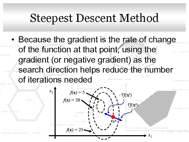Click to edit Master. Method Steepest Descent title style • Because the gradient is the rate of change of the function at that point, using the gradient (or negative gradient) as the search direction helps reduce the number of iterations needed x 2 f(x) = 5 - f(xk) f(x) = 20 f(xk) xk f(x) = 25 x 1

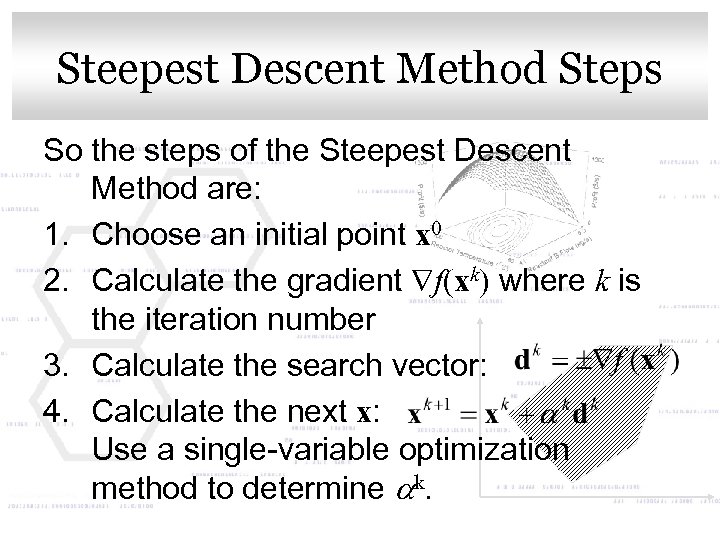Steepest Descent Method style Click to edit Master title Steps So the steps of the Steepest Descent Method are: 1. Choose an initial point x 0 2. Calculate the gradient f(xk) where k is the iteration number 3. Calculate the search vector: 4. Calculate the next x: Use a single-variable optimization method to determine ak.

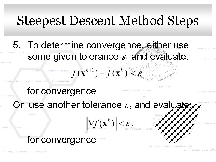Steepest Descent Method style Click to edit Master title Steps 5. To determine convergence, either use some given tolerance e 1 and evaluate: for convergence Or, use another tolerance e 2 and evaluate: for convergence

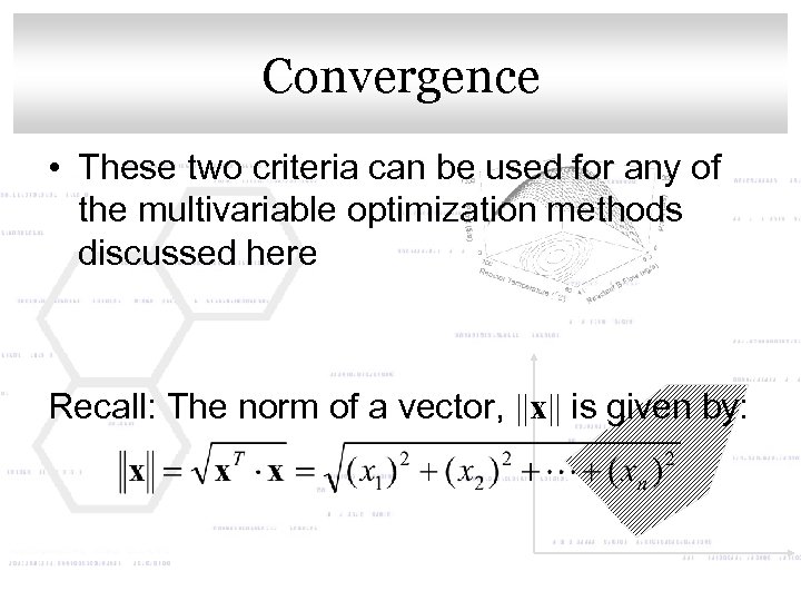Click to edit Master title style Convergence • These two criteria can be used for any of the multivariable optimization methods discussed here Recall: The norm of a vector, ||x|| is given by:

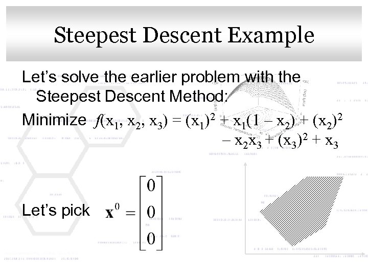Click to edit Master title style Steepest Descent Example Let’s solve the earlier problem with the Steepest Descent Method: Minimize f(x 1, x 2, x 3) = (x 1)2 + x 1(1 – x 2) + (x 2)2 – x 2 x 3 + (x 3)2 + x 3 Let’s pick

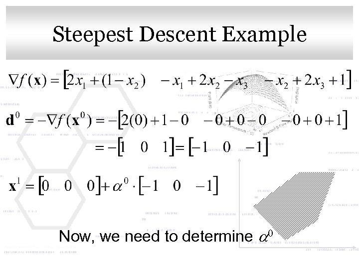Click to edit Master title style Steepest Descent Example Now, we need to determine a 0

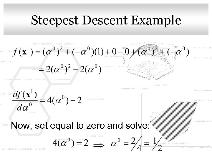Click to edit Master title style Steepest Descent Example Now, set equal to zero and solve:

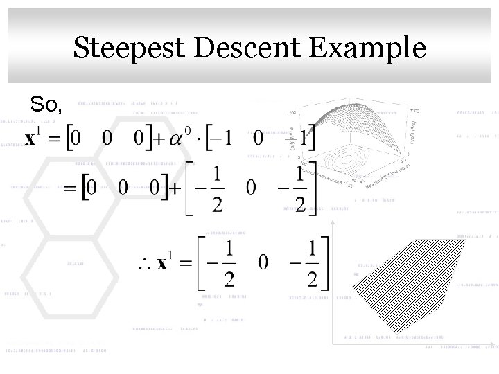Click to edit Master title style Steepest Descent Example So,

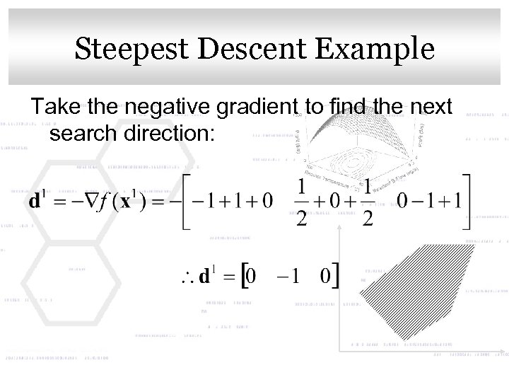Click to edit Master title style Steepest Descent Example Take the negative gradient to find the next search direction:

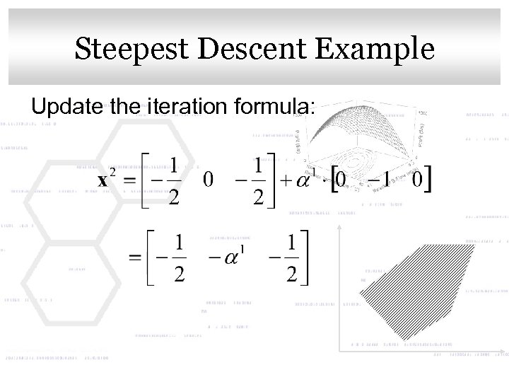Click to edit Master title style Steepest Descent Example Update the iteration formula:

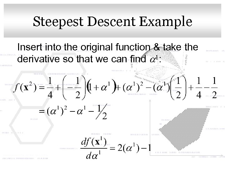Click to edit Master title style Steepest Descent Example Insert into the original function & take the derivative so that we can find a 1:

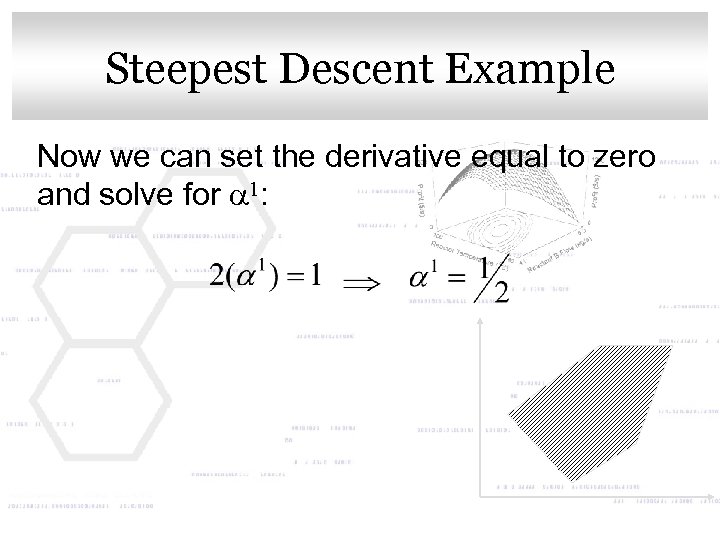Click to edit Master title style Steepest Descent Example Now we can set the derivative equal to zero and solve for a 1:

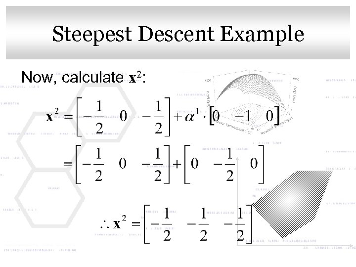Click to edit Master title style Steepest Descent Example Now, calculate x 2:

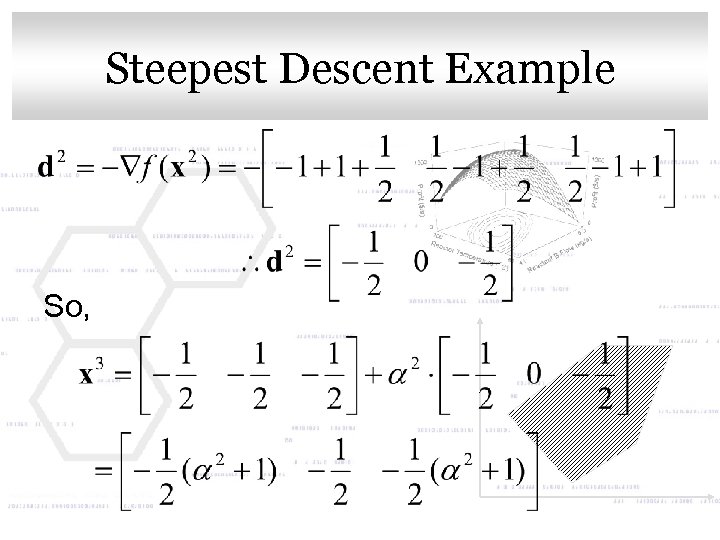Click to edit Master title style Steepest Descent Example So,

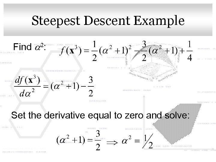Click to edit Master title style Steepest Descent Example Find a 2: Set the derivative equal to zero and solve:

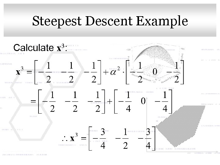Click to edit Master title style Steepest Descent Example Calculate x 3:

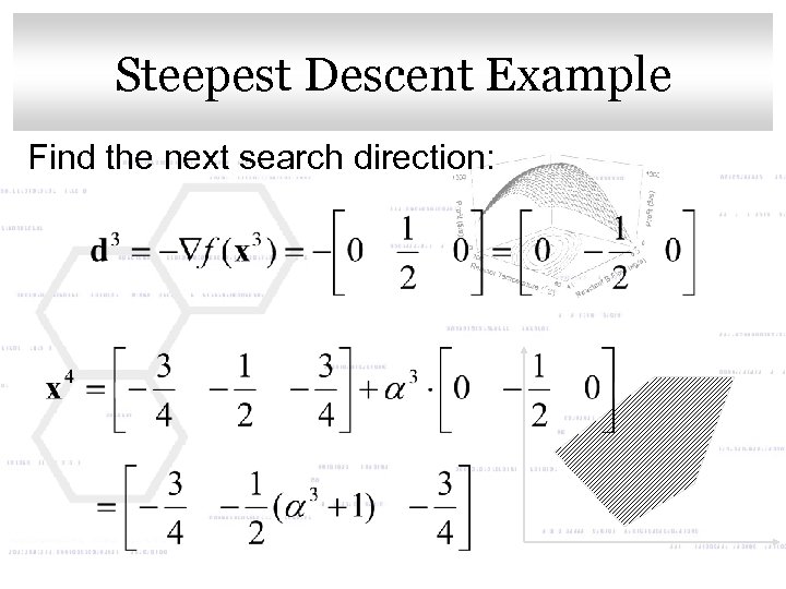Click to edit Master title style Steepest Descent Example Find the next search direction:

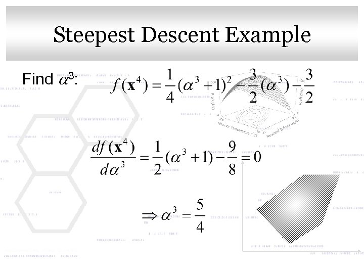Click to edit Master title style Steepest Descent Example Find a 3:

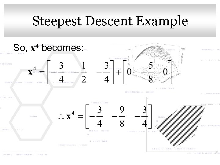Click to edit Master title style Steepest Descent Example So, x 4 becomes:

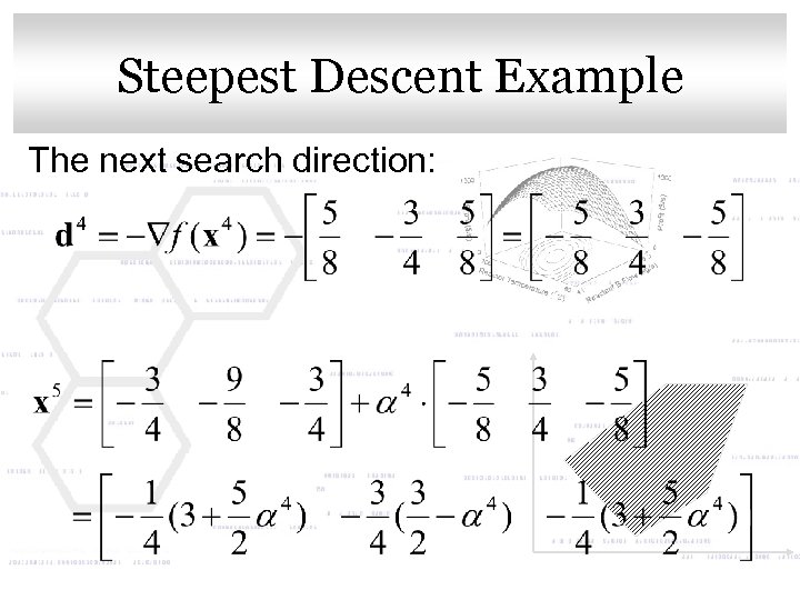Click to edit Master title style Steepest Descent Example The next search direction:

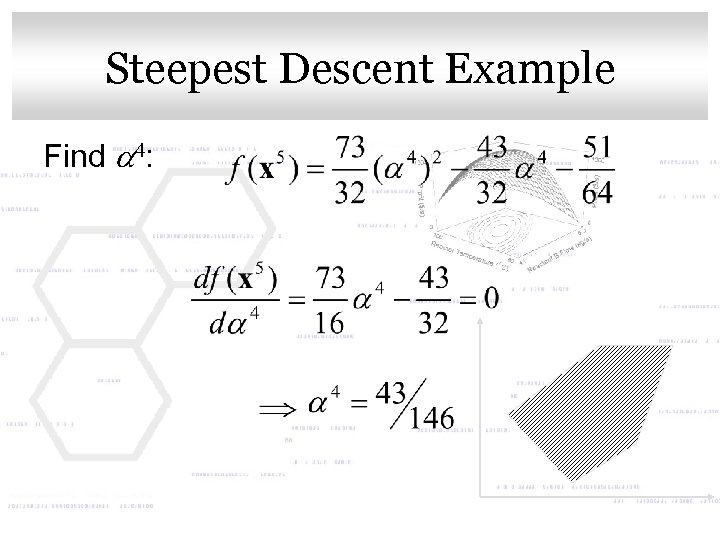Click to edit Master title style Steepest Descent Example Find a 4:

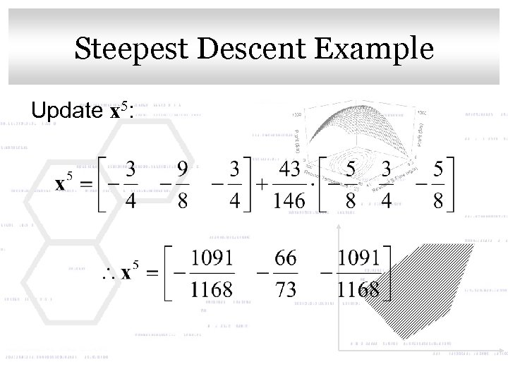Click to edit Master title style Steepest Descent Example Update x 5:

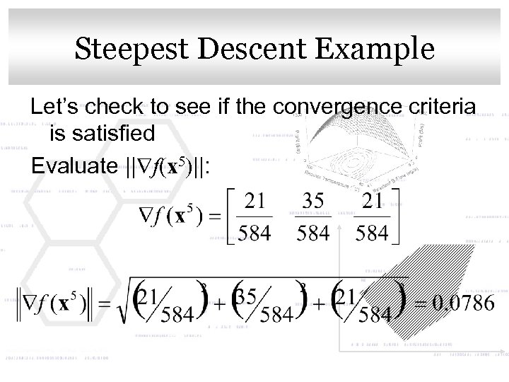Click to edit Master title style Steepest Descent Example Let’s check to see if the convergence criteria is satisfied Evaluate || f(x 5)||:

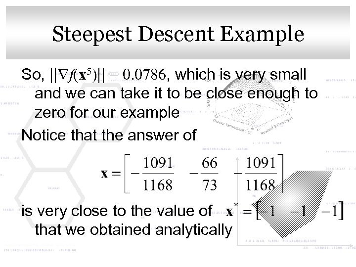Click to edit Master title style Steepest Descent Example So, || f(x 5)|| = 0. 0786, which is very small and we can take it to be close enough to zero for our example Notice that the answer of is very close to the value of that we obtained analytically

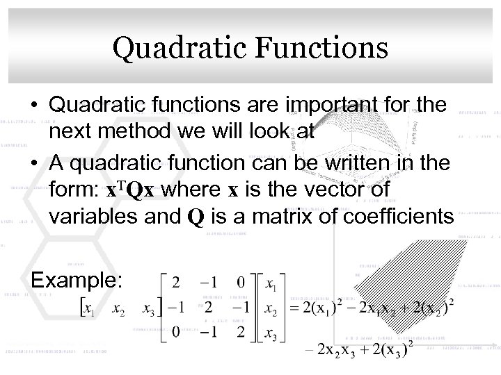Click to edit Master title style Quadratic Functions • Quadratic functions are important for the next method we will look at • A quadratic function can be written in the form: x. TQx where x is the vector of variables and Q is a matrix of coefficients Example:

Click to edit Master title style Conjugate Gradient Method • The Conjugate Gradient Method has the property that if f(x) is quadratic, it will take exactly n iterations to converge, where n is the number of variables in the x vector • Although it works especially well with quadratic functions, this method will work with non-quadratic functions also

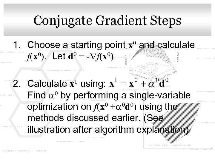Click to edit Master title style Conjugate Gradient Steps 1. Choose a starting point x 0 and calculate f(x 0). Let d 0 = - f(x 0) 2. Calculate x 1 using: Find a 0 by performing a single-variable optimization on f(x 0 +a 0 d 0) using the methods discussed earlier. (See illustration after algorithm explanation)

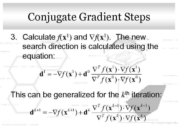Click to edit Master title style Conjugate Gradient Steps 3. Calculate f(x 1) and f(x 1). The new search direction is calculated using the equation: This can be generalized for the kth iteration:

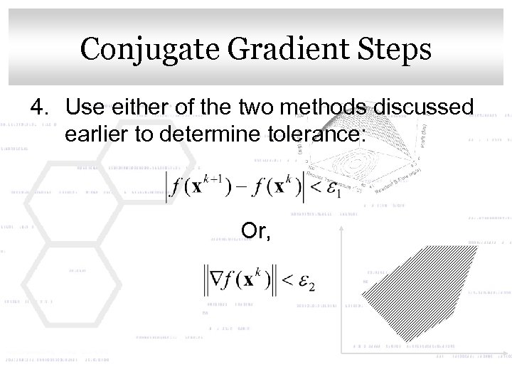Click to edit Master title style Conjugate Gradient Steps 4. Use either of the two methods discussed earlier to determine tolerance: Or,

Click to edit Master title style Number of Iterations • For quadratic functions, this method will converge in n iterations (k = n) • For non-quadratic functions, after n iterations, the algorithm cycles again with dn+1 becoming d 0.

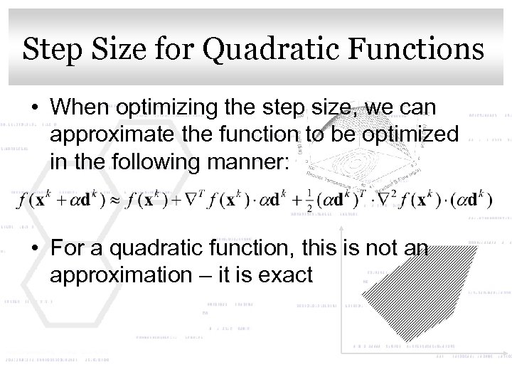Step Size for Quadratic Functions Click to edit Master title style • When optimizing the step size, we can approximate the function to be optimized in the following manner: • For a quadratic function, this is not an approximation – it is exact

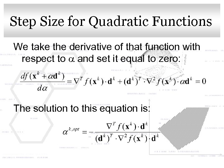Step Size for Quadratic Functions Click to edit Master title style We take the derivative of that function with respect to a and set it equal to zero: The solution to this equation is:

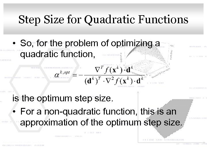Step Size for Quadratictitle style Click to edit Master Functions • So, for the problem of optimizing a quadratic function, is the optimum step size. • For a non-quadratic function, this is an approximation of the optimum step size.

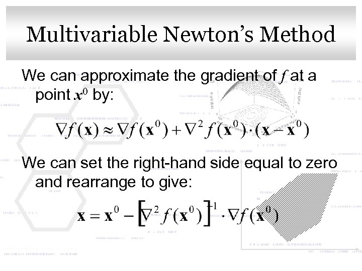Multivariable Master title style Click to edit Newton’s Method We can approximate the gradient of f at a point x 0 by: We can set the right-hand side equal to zero and rearrange to give:

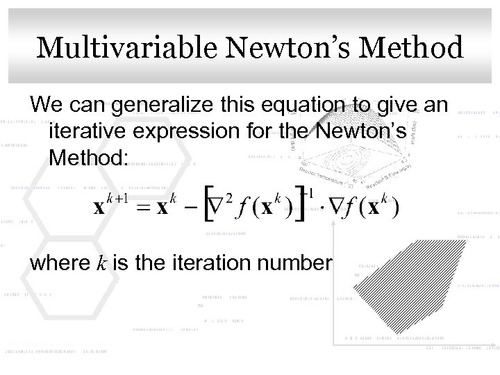Multivariable Master title style Click to edit Newton’s Method We can generalize this equation to give an iterative expression for the Newton’s Method: where k is the iteration number

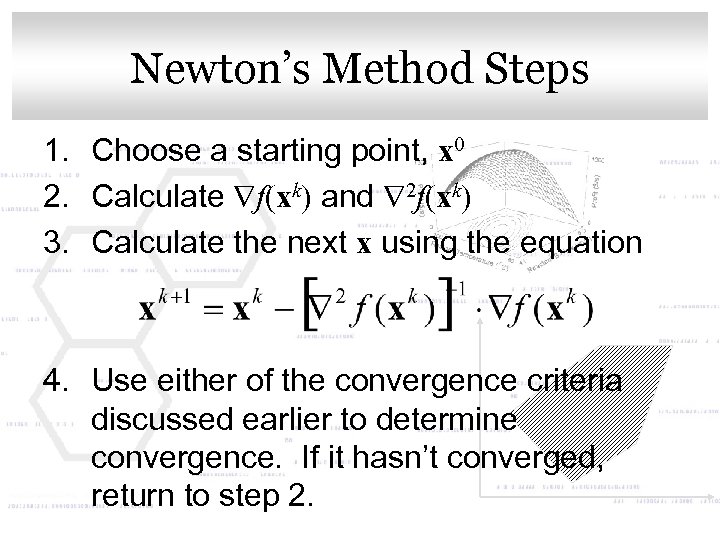Click to edit Master title style Newton’s Method Steps 1. Choose a starting point, x 0 2. Calculate f(xk) and 2 f(xk) 3. Calculate the next x using the equation 4. Use either of the convergence criteria discussed earlier to determine convergence. If it hasn’t converged, return to step 2.

Comments on. Master title style Click to edit Newton’s Method • We can see that unlike the previous two methods, Newton’s Method uses both the gradient and the Hessian • This usually reduces the number of iterations needed, but increases the computation needed for each iteration • So, for very complex functions, a simpler method is usually faster

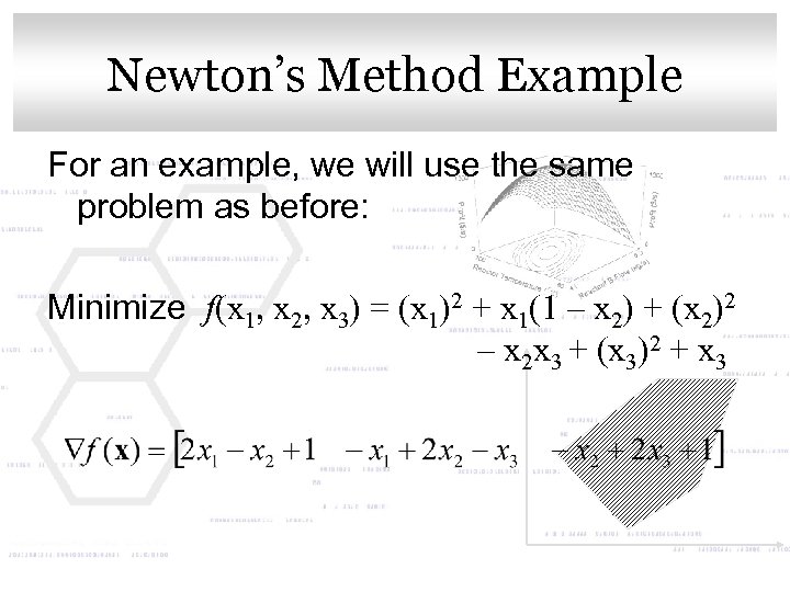Click to edit Master. Example Newton’s Method title style For an example, we will use the same problem as before: Minimize f(x 1, x 2, x 3) = (x 1)2 + x 1(1 – x 2) + (x 2)2 – x 2 x 3 + (x 3)2 + x 3

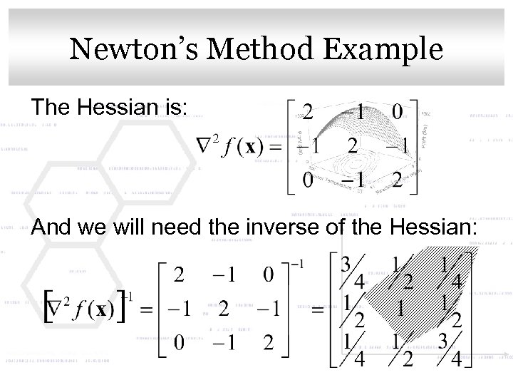Click to edit Master. Example Newton’s Method title style The Hessian is: And we will need the inverse of the Hessian:

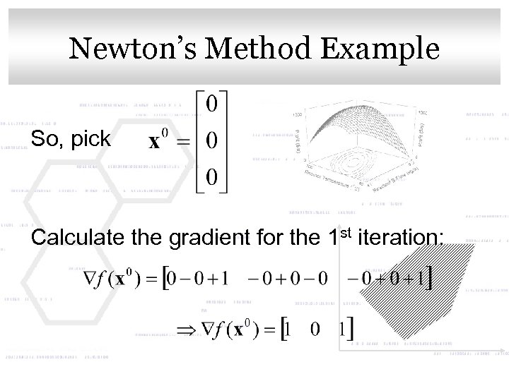Click to edit Master. Example Newton’s Method title style So, pick Calculate the gradient for the 1 st iteration:

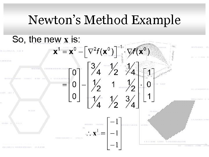Click to edit Master. Example Newton’s Method title style So, the new x is:

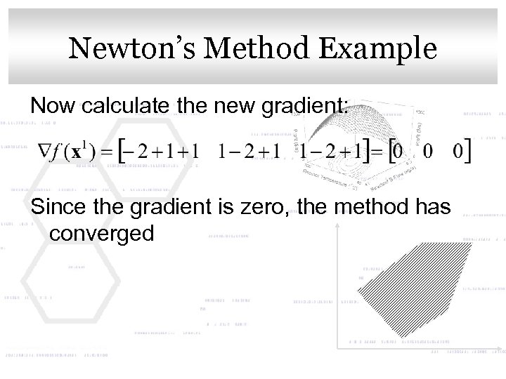Click to edit Master. Example Newton’s Method title style Now calculate the new gradient: Since the gradient is zero, the method has converged

Click to edit Master title style Comments on Example • Because it uses the 2 nd derivative, Newton’s Method models quadratic functions exactly and can find the optimum point in one iteration. • If the function had been a higher order, the Hessian would not have been constant and it would have been much more work to calculate the Hessian and take the inverse for each iteration.

Constrained Nonlinear Click to edit Master title style Optimization • Previously in this chapter, we solved NLP problems that only had objective functions, with no constraints. • Now we will look at methods on how to solve problems that include constraints.

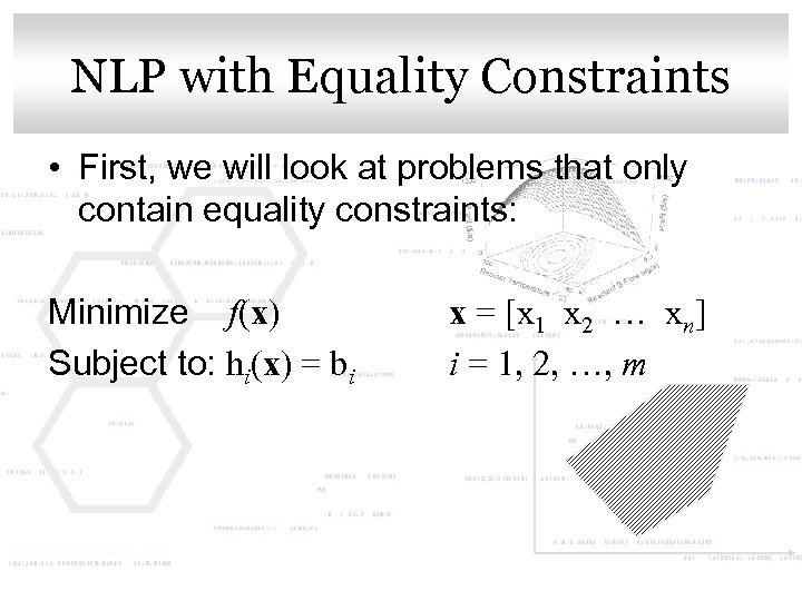NLP with Equality Constraints Click to edit Master title style • First, we will look at problems that only contain equality constraints: Minimize f(x) Subject to: hi(x) = bi x = [x 1 x 2 … xn] i = 1, 2, …, m

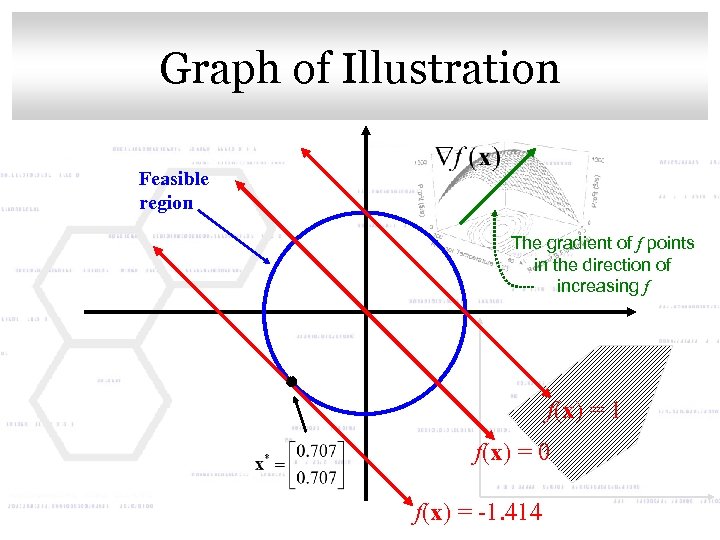
Click to edit Master title style Illustration Consider the problem: Minimize x 1 + x 2 Subject to: (x 1)2 + (x 2)2 – 1 = 0 The feasible region is a circle with a radius of one. The possible objective function curves are lines with a slope of -1. The minimum will be the point where the lowest line still touches the circle.

Click to edit Master title style Graph of Illustration Feasible region The gradient of f points in the direction of increasing f f(x) = 1 f(x) = 0 f(x) = -1. 414

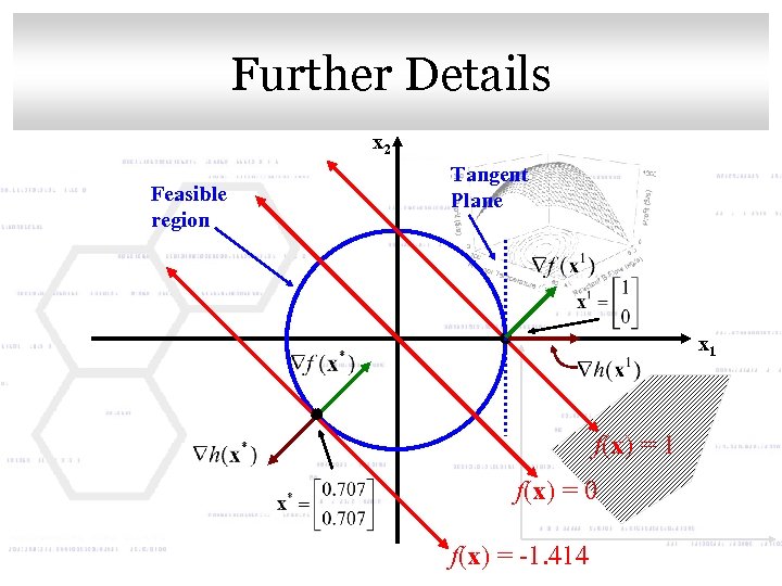
Click. More on the Graph style to edit Master title • Since the objective function lines are straight parallel lines, the gradient of f is a straight line pointing toward the direction of increasing f, which is to the upper right • The gradient of h will be pointing out from the circle and so its direction will depend on the point at which the gradient is evaluated.

Click to edit Master title style Further Details x 2 Feasible region Tangent Plane x 1 f(x) = 0 f(x) = -1. 414

Click to edit Master title style Conclusions • At the optimum point, f(x) is perpendicular to h(x) • As we can see at point x 1, f(x) is not perpendicular to h(x) and we can move (down) to improve the objective function • We can say that at a max or min, f(x) must be perpendicular to h(x) – Otherwise, we could improve the objective function by changing position

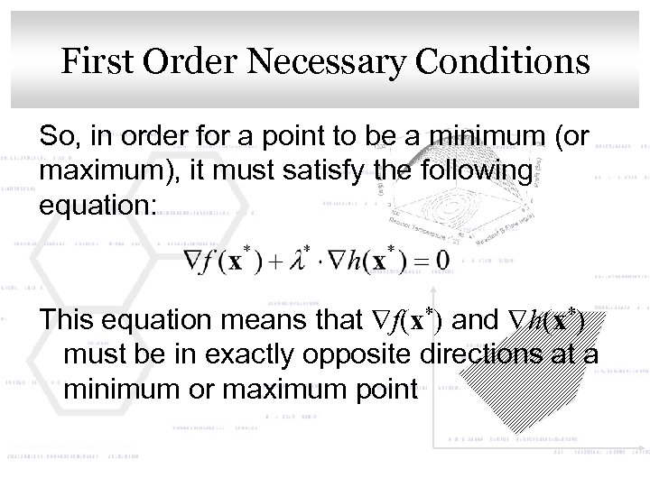First Order Necessary Conditions Click to edit Master title style So, in order for a point to be a minimum (or maximum), it must satisfy the following equation: This equation means that f(x*) and h(x*) must be in exactly opposite directions at a minimum or maximum point

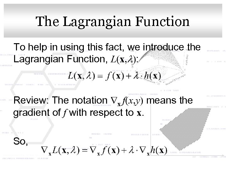Click to edit Master title style The Lagrangian Function To help in using this fact, we introduce the Lagrangian Function, L(x, l): Review: The notation x f(x, y) means the gradient of f with respect to x. So,

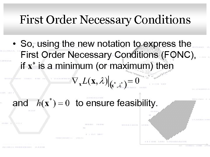First Order Necessary Conditions Click to edit Master title style • So, using the new notation to express the First Order Necessary Conditions (FONC), if x* is a minimum (or maximum) then and to ensure feasibility.

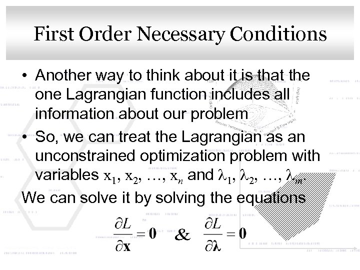First Order Necessary Conditions Click to edit Master title style • Another way to think about it is that the one Lagrangian function includes all information about our problem • So, we can treat the Lagrangian as an unconstrained optimization problem with variables x 1, x 2, …, xn and l 1, l 2, …, lm. We can solve it by solving the equations

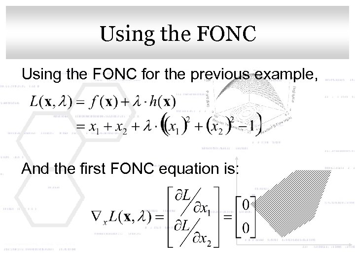Click to edit Master title style Using the FONC for the previous example, And the first FONC equation is:

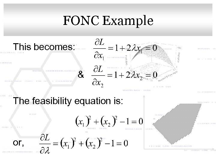Click to edit Master title style FONC Example This becomes: & The feasibility equation is: or,

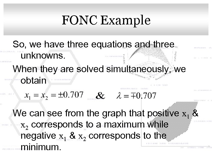Click to edit Master title style FONC Example So, we have three equations and three unknowns. When they are solved simultaneously, we obtain We can see from the graph that positive x 1 & x 2 corresponds to a maximum while negative x 1 & x 2 corresponds to the minimum.

Click. FONC Observationsstyle to edit Master title • If you go back to the LP Chapter and look at the mathematical definition of the KKT conditions, you may notice that they look just like our FONC that we just used • This is because it is the same concept • We simply used a slightly different derivation this time but obtained the same result

Click to edit Master title style Limitations of FONC • The FONC do not guarantee that the solution(s) will be minimums/maximums. • As in the case of unconstrained optimization, they only provide us with candidate points that need to be verified by the second order conditions. • Only if the problem is convex do the FONC guarantee the solutions will be extreme points.

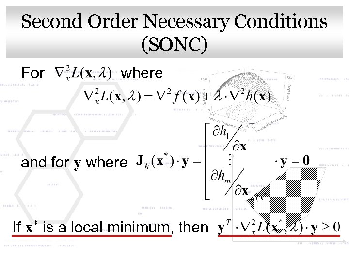Second Order Necessary Conditions Click to edit Master title style (SONC) For where and for y where If x* is a local minimum, then

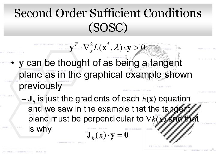Second Order Sufficient Conditions Click to edit Master title style (SOSC) • y can be thought of as being a tangent plane as in the graphical example shown previously – Jh is just the gradients of each h(x) equation and we saw in the example that the tangent plane must be perpendicular to h(x) and that is why

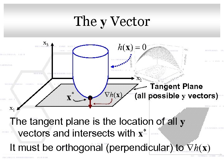The y Vector Click to edit Master title style x 3 x 2 Tangent Plane (all possible y vectors) x 1 The tangent plane is the location of all y vectors and intersects with x* It must be orthogonal (perpendicular) to h(x)

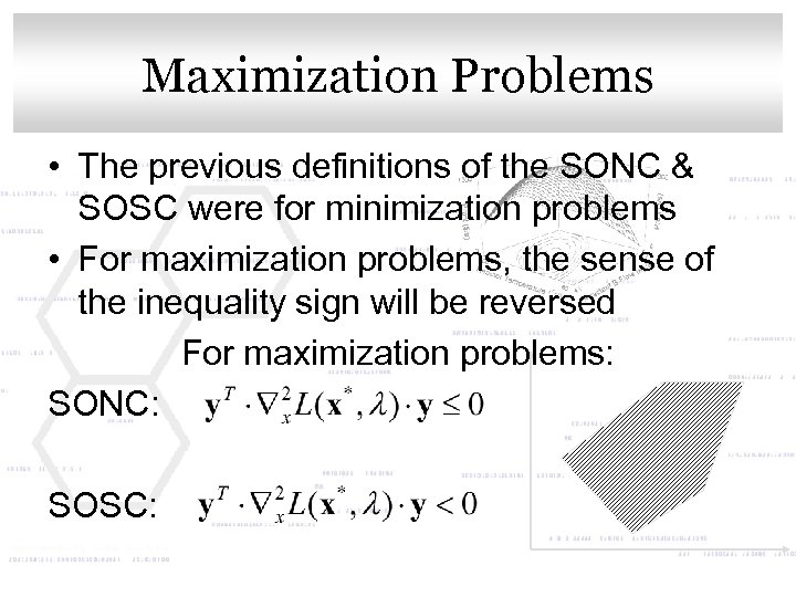Click to edit Master title style Maximization Problems • The previous definitions of the SONC & SOSC were for minimization problems • For maximization problems, the sense of the inequality sign will be reversed For maximization problems: SONC: SOSC:

Click to edit Master title style Necessary & Sufficient • The necessary conditions are required for a point to be an extremum but even if they are satisfied, they do not guarantee that the point is an extremum. • If the sufficient conditions are true, then the point is guaranteed to be an extremum. But if they are not satisfied, this does not mean that the point is not an extremum.

Click to edit Master title style Procedure 1. Solve the FONC to obtain candidate points. 2. Test the candidate points with the SONC – Eliminate any points that do not satisfy the SONC 3. Test the remaining points with the SOSC – The points that satisfy them are min/max’s – For the points that do not satisfy, we cannot say whether they are extreme points or not

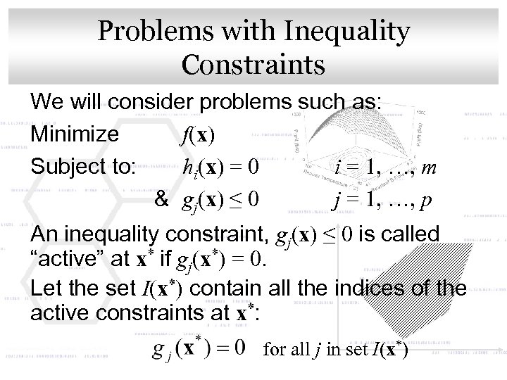Problems with Inequality Click to edit Master title style Constraints We will consider problems such as: Minimize f(x) Subject to: hi(x) = 0 i = 1, …, m & gj(x) ≤ 0 j = 1, …, p An inequality constraint, gj(x) ≤ 0 is called “active” at x* if gj(x*) = 0. Let the set I(x*) contain all the indices of the active constraints at x*: for all j in set I(x*)

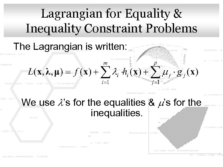Lagrangian for Equality & Click to edit Master title style Inequality Constraint Problems The Lagrangian is written: We use l’s for the equalities & m’s for the inequalities.

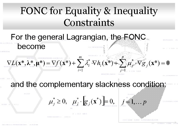FONC for Equality & Inequality Click to edit Master title style Constraints For the general Lagrangian, the FONC become and the complementary slackness condition:

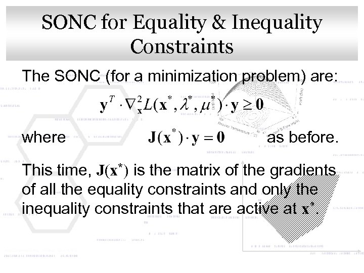SONC for Equality & Inequality Click to edit Master title style Constraints The SONC (for a minimization problem) are: where as before. This time, J(x*) is the matrix of the gradients of all the equality constraints and only the inequality constraints that are active at x*.

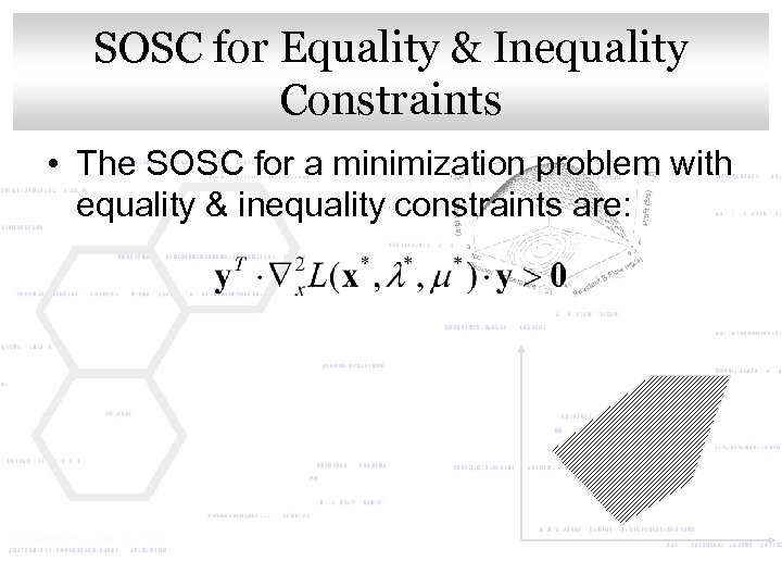SOSC for Equality & Inequality Click to edit Master title style Constraints • The SOSC for a minimization problem with equality & inequality constraints are:

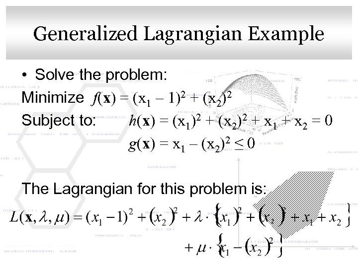Generalized Lagrangian Example Click to edit Master title style • Solve the problem: Minimize f(x) = (x 1 – 1)2 + (x 2)2 Subject to: h(x) = (x 1)2 + (x 2)2 + x 1 + x 2 = 0 g(x) = x 1 – (x 2)2 ≤ 0 The Lagrangian for this problem is:

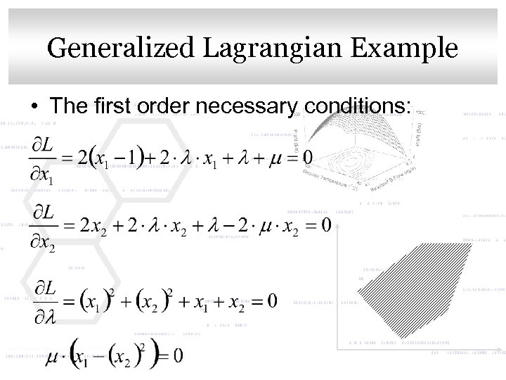Generalized Lagrangian Example Click to edit Master title style • The first order necessary conditions:

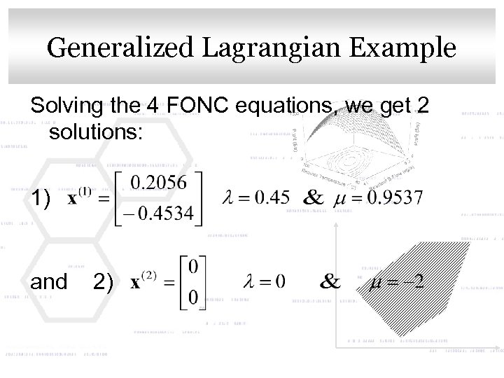Generalized Lagrangian Example Click to edit Master title style Solving the 4 FONC equations, we get 2 solutions: 1) and 2)

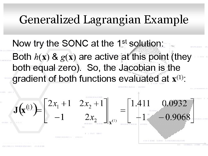Generalized Lagrangian Example Click to edit Master title style Now try the SONC at the 1 st solution: Both h(x) & g(x) are active at this point (they both equal zero). So, the Jacobian is the gradient of both functions evaluated at x(1):

Generalized Lagrangian Example Click to edit Master title style The only solution to the equation: is: And the Hessian of the Lagrangian is:

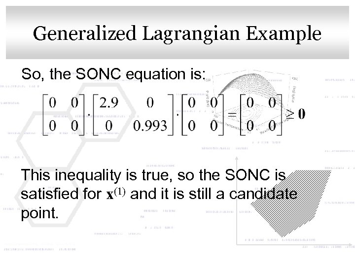Generalized Lagrangian Example Click to edit Master title style So, the SONC equation is: This inequality is true, so the SONC is satisfied for x(1) and it is still a candidate point.

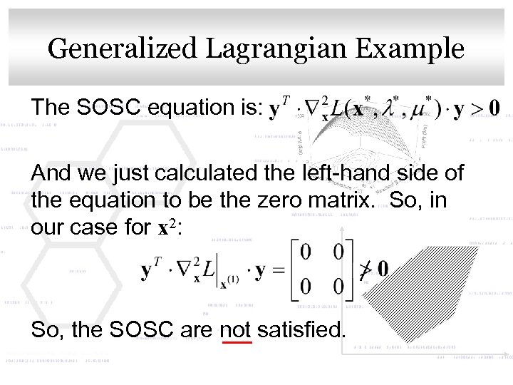Generalized Lagrangian Example Click to edit Master title style The SOSC equation is: And we just calculated the left-hand side of the equation to be the zero matrix. So, in our case for x 2: So, the SOSC are not satisfied.

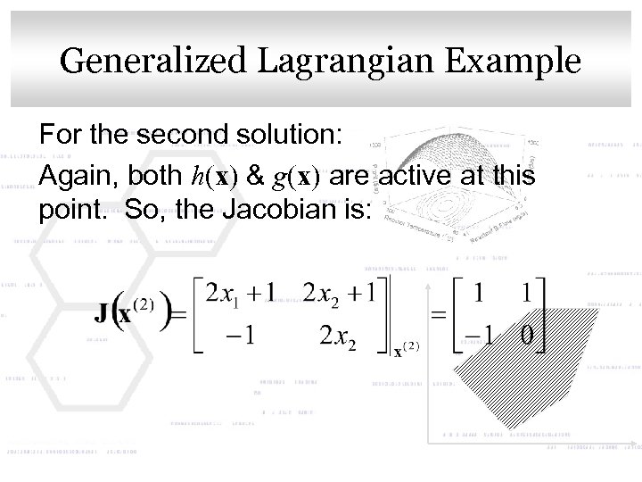Generalized Lagrangian Example Click to edit Master title style For the second solution: Again, both h(x) & g(x) are active at this point. So, the Jacobian is:

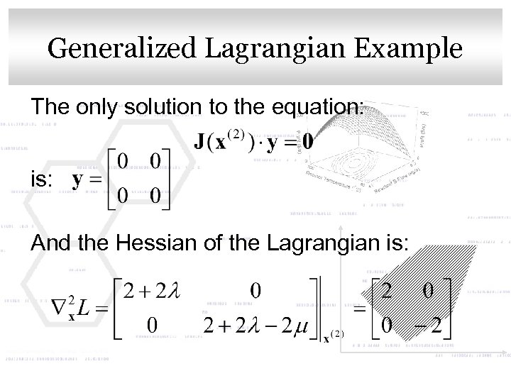Generalized Lagrangian Example Click to edit Master title style The only solution to the equation: is: And the Hessian of the Lagrangian is:

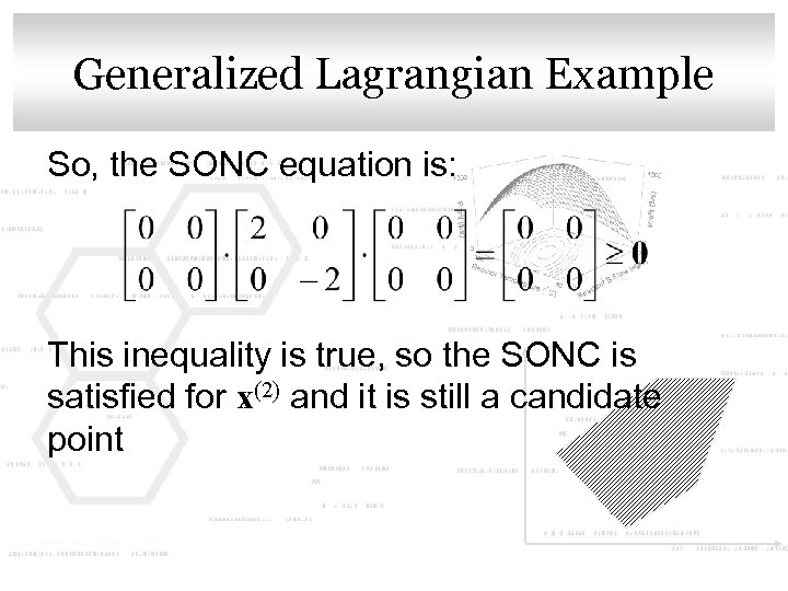Generalized Lagrangian Example Click to edit Master title style So, the SONC equation is: This inequality is true, so the SONC is satisfied for x(2) and it is still a candidate point

Generalized Lagrangian Example Click to edit Master title style The SOSC equation is: And we just calculated the left-hand side of the equation to be the zero matrix. So, in our case for x 2: So, the SOSC are not satisfied.

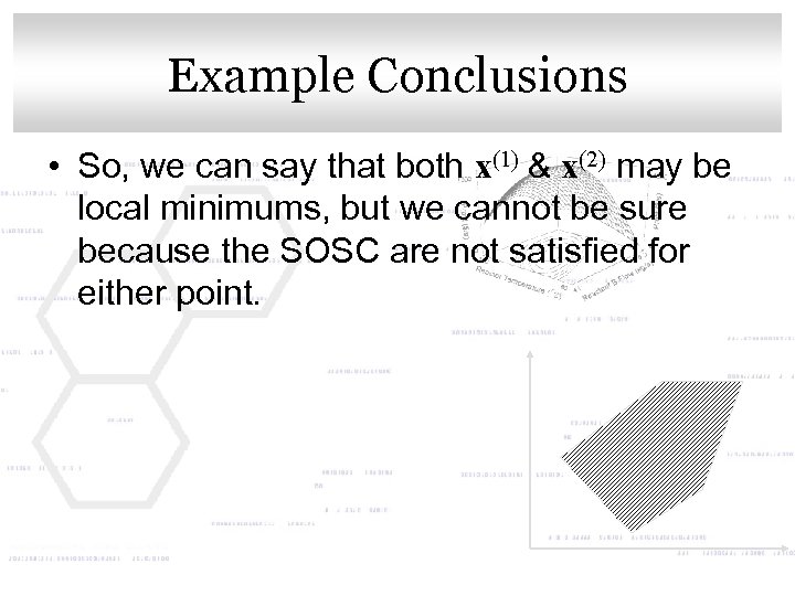Click to edit Master title style Example Conclusions • So, we can say that both x(1) & x(2) may be local minimums, but we cannot be sure because the SOSC are not satisfied for either point.

Click. Numerical Methodsstyle to edit Master title • As you can see from this example, the most difficult step is to solve a system of nonlinear equations to obtain the candidate points. • Instead of taking gradients of functions, automated NLP solvers use various methods to change a general NLP into an easier optimization problem.

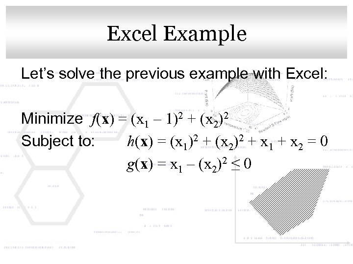Click to. Excel. Master title style edit Example Let’s solve the previous example with Excel: Minimize f(x) = (x 1 – 1)2 + (x 2)2 Subject to: h(x) = (x 1)2 + (x 2)2 + x 1 + x 2 = 0 g(x) = x 1 – (x 2)2 ≤ 0

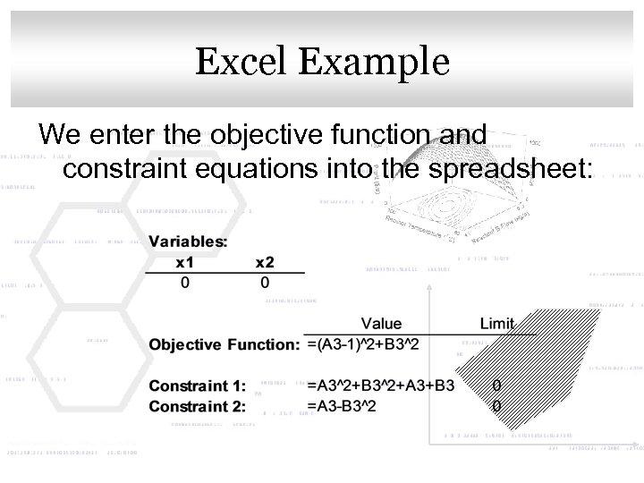Click to. Excel. Master title style edit Example We enter the objective function and constraint equations into the spreadsheet:

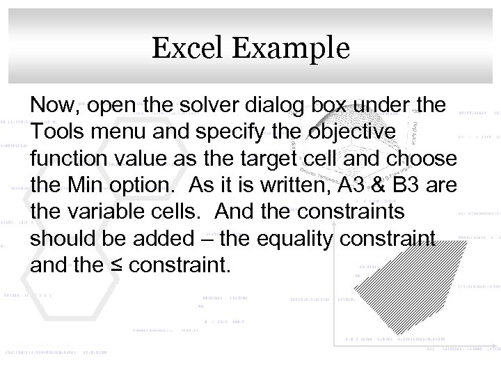Click to. Excel. Master title style edit Example Now, open the solver dialog box under the Tools menu and specify the objective function value as the target cell and choose the Min option. As it is written, A 3 & B 3 are the variable cells. And the constraints should be added – the equality constraint and the ≤ constraint.

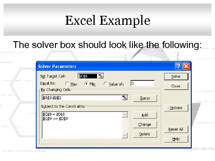Click to. Excel. Master title style edit Example The solver box should look like the following:

Click to. Excel. Master title style edit Example • This is a nonlinear model, so unlike the examples in the last chapter, we won’t choose the “Assume Linear Model” in the options menu • Also, x 1 & x 2 are not specified to be positive, so we don’t check the “Assume Non-negative” box • If desired, the tolerance may be decreased to 0. 1%

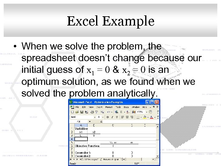Click to. Excel. Master title style edit Example • When we solve the problem, the spreadsheet doesn’t change because our initial guess of x 1 = 0 & x 2 = 0 is an optimum solution, as we found when we solved the problem analytically.

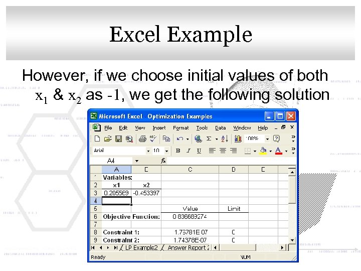Click to. Excel. Master title style edit Example However, if we choose initial values of both x 1 & x 2 as -1, we get the following solution

Click to edit Master title style Conclusions • So, by varying the initial values, we can get both of the candidate points we found previously • However, the NLP solver tells us that they are both local minimum points

Click to edit Master title style References Material for this chapter has been taken from: • Optimization of Chemical Processes 2 nd Ed. ; Edgar, Thomas; David Himmelblau; & Leon Lasdon.