5591850e76fb45a5dce49226b881b36a.ppt
- Количество слайдов: 53
 Tide Models The Navy sometimes uses the term “tide models” to designate those numerical ocean models being run primarily for the purpose of predicting tidal heights and/or currents. At this time, the tide models used by the Navy are run in a 2 D mode (no variation in the vertical dimension). By definition these models must include tidal forcing, but they may also include other types of forcing, just as other ocean circulation models used by the Navy may include tidal forcing.
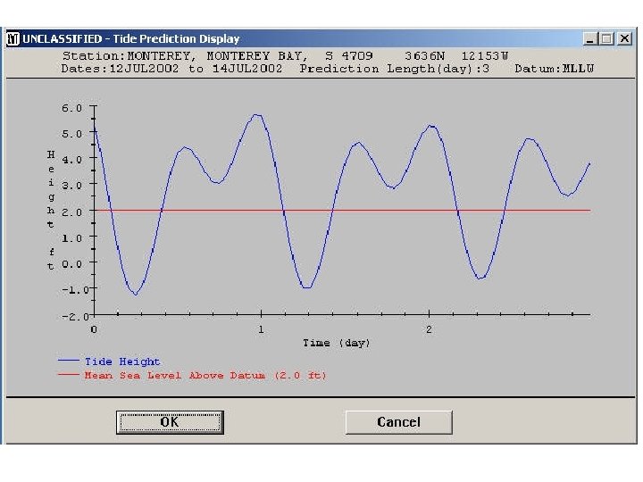
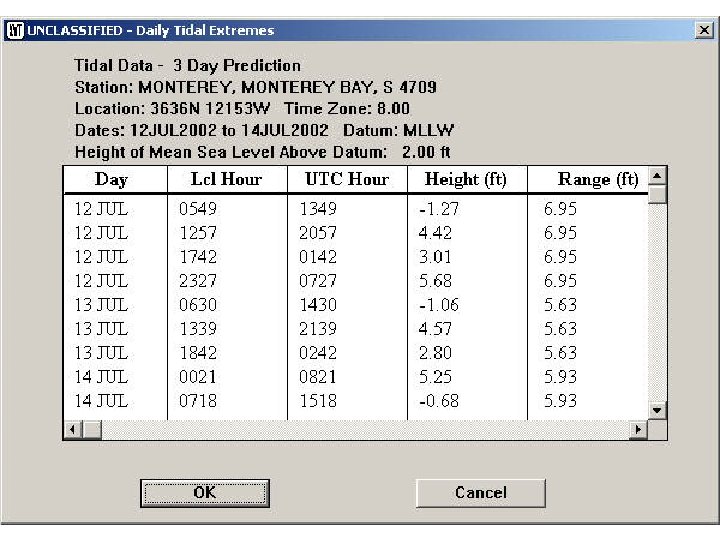
 GFMPL TP • The GFMPL Tide Prediction program is not an ocean model in the sense of the other models discussed in this course. • TP can predict hourly tidal heights at a fixed number of reference stations by using tidal constants (amplitude and phase) previously calculated from measurements made at those locations. • Additionally, it can predict tidal heights at a set of secondary stations, by applying known corrections to the reference stations.
 • Tidal heights may only be forecast at locations for which historical tidal data are available (i. e. , tide stations provided by the data base). • This method does not account for sea level variations due to changes in atmospheric pressure, nor those due to wind forcing. • Tidal currents are not predicted.
 ADCIRC Advanced Circulation model Primary contacts: Cheryl Ann Blain (NRL-SSC), Steve Haeger (NAVO) ADCIRC was developed in the late 1980’s to early 1990’s by Rick Luettich (Univ. of N. Carolina) and Joannes Westerink (Univ. of Notre Dame) in conjunction with the Coastal Engineering Research Center (now called the Engineering Research and Development Center) of the Army Corps of Engineers. It is currently used in a 2 D mode by NAVO for tidal and surge current and height predictions in littoral areas, although in the future, tidal currents may only be shown for those areas where the currents are dominated by tides. A 3 D version, though still barotropic, is available and a baroclinic version is under development.
 ADCIRC http: //www. marine. unc. edu/C_CATS/adcirc/ http: //www. nd. edu/~adcirc/ ADCIRC is a finite element, free surface barotropic ocean circulation model. NAVO runs the 2 D version with tidal and wind forcing, for the primary purpose of predicting sea level height. While sea level is not strongly influenced by density structure, currents may be, so tidal current forecasts are likely to be best where the water is well-mixed top to bottom.
 Physics • Shallow water equations, including nonlinear terms The equations have been formulated using the traditional hydrostatic pressure and Boussinesq approximations. A quadratic form of bottom friction is used. Although the drag coefficient may vary in space, it is generally specified as constant.
 Domain • Due to the complications in designing and implementing an efficient and accurate grid, NAVO runs ADCIRC only in a limited number of domains. It is technically feasible, but personnel-intensive. • NRL and others are working to implement an automated grid generation program so that ADCIRC can be rapidly relocated to new geographic areas. It is presently being used in a research, although not an operational, setting. • NAVO is currently running ADCIRC for three geographic regions: the Yellow Sea and Sea of Japan; the Arabian Gulf and Gulf of Oman; and the western North Atlantic Ocean including the Caribbean, Gulf of Mexico and US Eastern Seaboard.
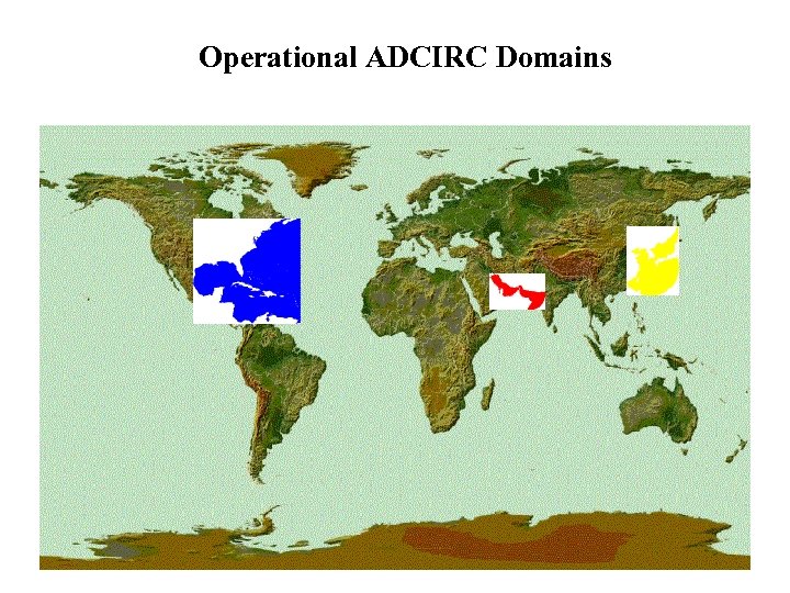 Operational ADCIRC Domains
 Grid and Coordinate System • ADCIRC uses a finite element grid in the horizontal. • ADCIRC may be run in either Cartesian or spherical coordinates. NAVO uses spherical coordinates. • Since it is 2 D, there is no vertical coordinate. The velocities are a depth-average.
 Spatial and Temporal Resolution • One of the advantages of a finite element grid, is that the spatial resolution is continuously variable over the domain. Generally it varies from a few 10’s of meters to several kilometers. • The model as implemented at NAVO uses a time step of 30 seconds.
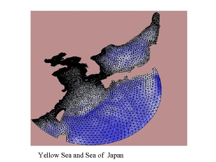 Yellow Sea and Sea of Japan
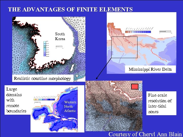 THE ADVANTAGES OF FINITE ELEMENTS South Korea Mississippi River Delta Realistic coastline morphology Large domains with remote boundaries Western North Atlantic Fine-scale resolution of inter-tidal zones Courtesy of Cheryl Ann Blain
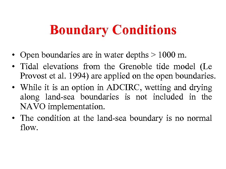 Boundary Conditions • Open boundaries are in water depths > 1000 m. • Tidal elevations from the Grenoble tide model (Le Provost et al. 1994) are applied on the open boundaries. • While it is an option in ADCIRC, wetting and drying along land-sea boundaries is not included in the NAVO implementation. • The condition at the land-sea boundary is no normal flow.
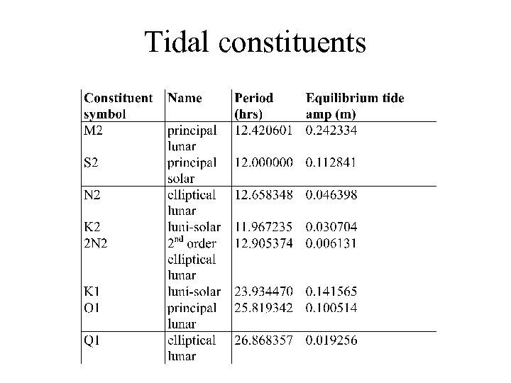 Tidal constituents
 Forcing • In addition to the tidal elevations applied on the open boundaries, astronomical tide generating forces are applied over the whole domain. • Atmospheric pressure and wind stress forcing from either NOGAPS (the western North Atlantic Ocean), COAMPSTM (the Yellow Sea and Sea of Japan) or a combination of the two (Arabian Gulf and Gulf of Oman) is used.
 Initialization • The model is started from rest. • The density is constant and uniform. • NAVO generally uses a spin-up time of 3 days before results are used. • A longer spin-up time is desirable. In the future, this might be accomplished by changes in the implementation, and/or taking advantage of a warm start capability after a long initial spin-up.
 Data Assimilation • No data is assimilated into this model.
 Implementation • Can be executed on all super-computer and workstation platforms. • Computationally efficient.
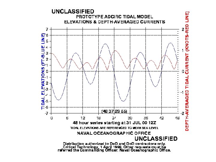
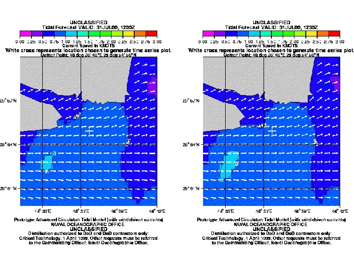
 Output • Tidal heights and currents are output at 30 min intervals for a 48 -hr forecast. • The numerical output is post-processed to produce a graphical format. The graphics generally do not show the whole domain, but rather are focused on predetermined areas of the grid. This may affect how the results are interpreted.
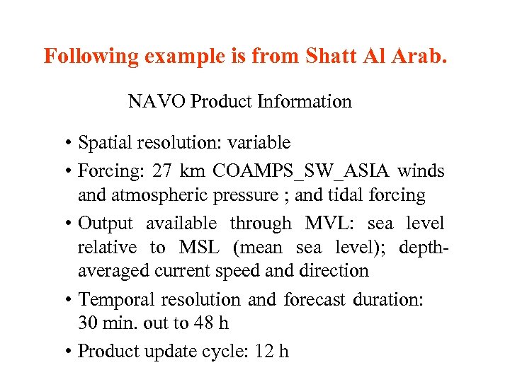 Following example is from Shatt Al Arab. NAVO Product Information • Spatial resolution: variable • Forcing: 27 km COAMPS_SW_ASIA winds and atmospheric pressure ; and tidal forcing • Output available through MVL: sea level relative to MSL (mean sea level); depthaveraged current speed and direction • Temporal resolution and forecast duration: 30 min. out to 48 h • Product update cycle: 12 h
 Arabian Gulf Yellow Sea
 References Blain, C. A. , R. H. Preller, and A. P. Rivera, Tidal prediction using the Advanced Circulation Model (ADCIRC) and a relocatable PC-based system, Oceanography, 15 (1), 77 -87, 2002. Luettich, R. , and J. Westerink, Users Manual: ADCIRC, A (Parallel) Advanced Circulation Model for Oceanic, Coastal and Estuarine Waters, http: //www. marine. unc. edu/C_CATS/adcirc/, 2000.
 PCTides Primary contacts: Ruth Preller, NRL-SSC • Over the past 3 years, NRL has developed a globally relocatable tide/surge prediction capability, designed for use on or near continental shelves. • “The capability is utilized for locations where neither observations nor a regularly run operational tide prediction model, such as ADCIRC, exists. ” (Blain et al. 2002).
 PCTides http: //www 7320. nrlssc. navy. mil/pctides/ • “PCTides is the NRL’s globally relocatable tide/surge forecast system used for the rapid prediction of tidal amplitude and phase, as well as barotropic ocean currents. ” • There are 2 D and 3 D versions, both based on the shallow water equations. Normally the 2 D version is used. • “All databases, except for the wind forcing, are internal to the PCTides system. ” (All quotations in this section are taken from the web site listed above, unless otherwise noted. )
 Physics • PCTides includes 2 tide/surge models: the Global Environmental Modeling Services (GEMS) Coastal Ocean Model (GCOM 2 D and GCOM 3 D). • GCOM 2 D is a depth-integrated, barotropic hydrodynamic model. It solves for SSH and mean current structure (i. e. no vertical variation). • GCOM 3 D allows for vertical variations in the currents. It can be run in either barotropic mode (no thermal or density variation), or baroclinic mode (solves for temperature and salinity). The baroclinic mode is not generally available, and will not be discussed here. • A wetting and drying algorithm for simulation of coastal flooding is included.
 Domain • Selected by the user, using a rubberbanding method through the GUI or by entering latitude/longitude limits. • Domains may be nested within one another to achieve higher spatial resolution in the inner domain.
 Grid and Coordinate System • The version most commonly used by Navy METOC is 2 D, so has no vertical coordinate. • The 3 D version uses a z-coordinate system in the vertical. • A Cartesian grid is used in the horizontal plane, with C type finite differencing. • Grid arrays are constructed such that there are no more than 40, 000 grid points (e. g. 200 x 200). This keeps simulations fast, while still allowing for large enough regions with fine enough resolution.
 Spatial Resolution • Selected by the user through the GUI • Generally from 1 to 10 km • Bathymetry and open boundary conditions are automatically interpolated to the domain and grid selected by the user.
 Temporal resolution • To optimize efficiency, different time steps are used to solve different aspects of the equations. • The continuity equation and gravity wave and Coriolis terms use the shortest time step. • The nonlinear advection terms use an intermediate time step. • The surface and bottom stress terms are solved using the longest time step.
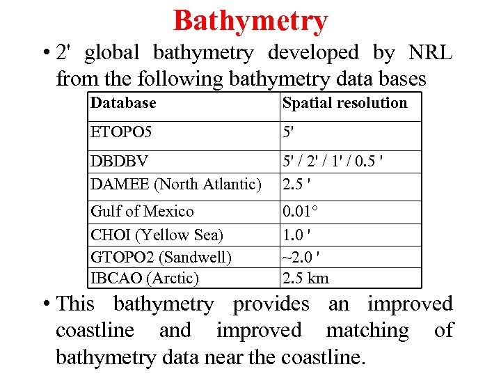 Bathymetry • 2' global bathymetry developed by NRL from the following bathymetry data bases Database Spatial resolution ETOPO 5 5' DBDBV DAMEE (North Atlantic) 5' / 2' / 1' / 0. 5 ' 2. 5 ' Gulf of Mexico CHOI (Yellow Sea) GTOPO 2 (Sandwell) IBCAO (Arctic) 0. 01° 1. 0 ' ~2. 0 ' 2. 5 km • This bathymetry provides an improved coastline and improved matching of bathymetry data near the coastline.
 Boundary Conditions • Included in PCTides are the Finite Element Solutions 95. 1/2. 1 (Shum et al. 1997) from the Grenoble global tide model (the same as those used for ADCIRC). These are used to provide sea surface displacements at the open boundaries of the ocean model. • The same 8 tidal constituents as used for ADCIRC are used for PCTides. • Atmospheric barometric displacement (change in sea level due to atmospheric pressure) is also specified at the open boundaries.
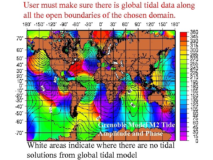 User must make sure there is global tidal data along all the open boundaries of the chosen domain. Grenoble Model M 2 Tide: Amplitude and Phase White areas indicate where there are no tidal solutions from global tidal model
 Forcing • The model may be driven by astronomical tidal forcing (through the open boundaries) and / or surface winds and pressures. • Winds and pressures may be entered manually (in which case they are uniform over the domain), or obtained from NOGAPS, COAMPSTM, or DAMPS through Met. Cast.
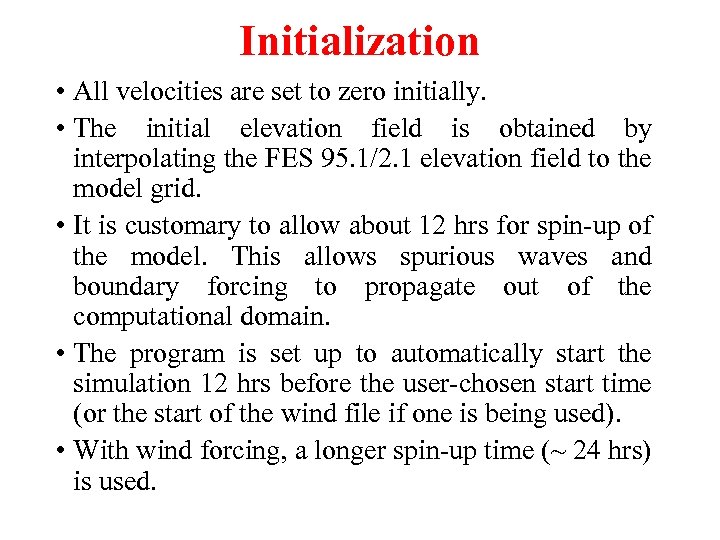 Initialization • All velocities are set to zero initially. • The initial elevation field is obtained by interpolating the FES 95. 1/2. 1 elevation field to the model grid. • It is customary to allow about 12 hrs for spin-up of the model. This allows spurious waves and boundary forcing to propagate out of the computational domain. • The program is set up to automatically start the simulation 12 hrs before the user-chosen start time (or the start of the wind file if one is being used). • With wind forcing, a longer spin-up time (~ 24 hrs) is used.
 Data Assimilation • Sea level variations from measurements made at the ~4500 International Hydrographic Office tidal stations are included in a PCTides database, and are used to constrain the solutions by using a weighted nudging approach described in Hubbert et al. 2001 (Blain et al. 2002).
 Implementation • Can be run on PCs and UNIX systems. • “The average PCTides 48 hour forecast takes anywhere from 3 to 10 minutes of run time on a 500 MHz PC. ” (Blain et al. 2002)
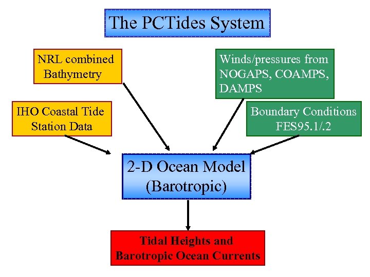 The PCTides System NRL combined Bathymetry Winds/pressures from NOGAPS, COAMPS, DAMPS IHO Coastal Tide Station Data Boundary Conditions FES 95. 1/. 2 2 -D Ocean Model (Barotropic) Tidal Heights and Barotropic Ocean Currents
 Output • Results may be output in graphical or text format. • Time series, with a time step typically of 10 -12 min, of sea level and currents are output at userspecified station locations. • Spatial fields of velocity and sea level are output at a user-specified time interval (the minimum interval is 30 min). • The length of the forecast is determined by the user, or the length of the wind forecast if one is being used. • The sea level deviations output must be added to a specified reference level (such as mean sea level) to get actual water depths.
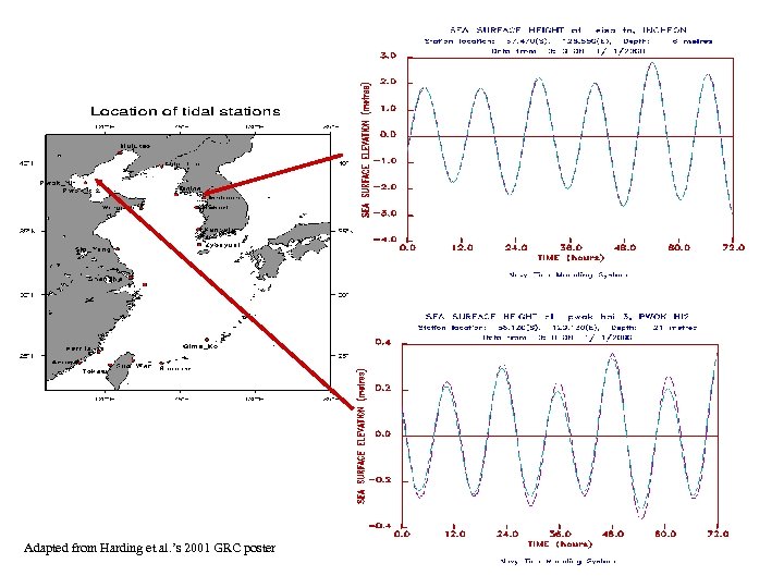 Adapted from Harding et al. ’s 2001 GRC poster
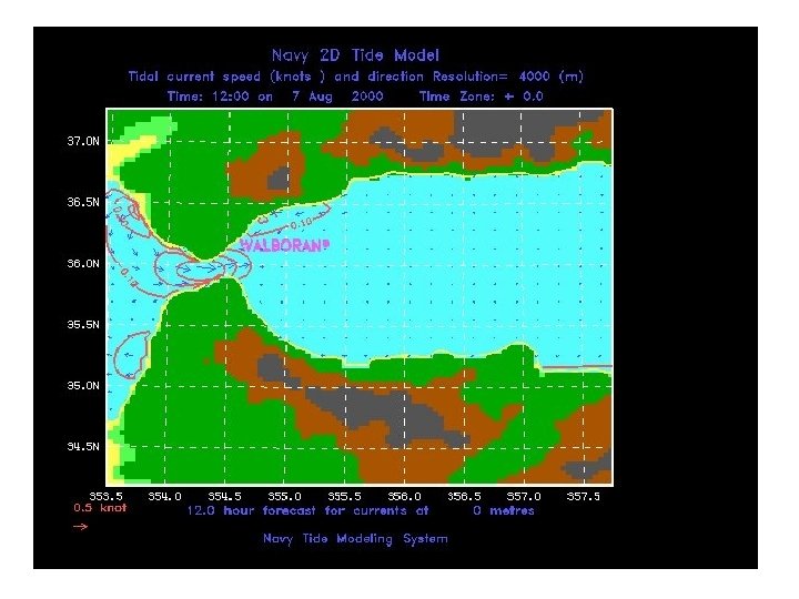
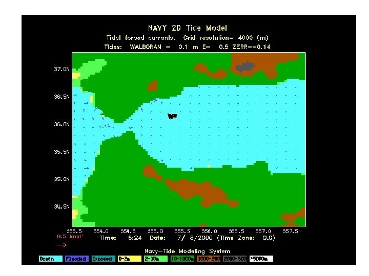
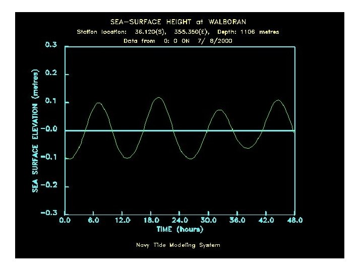
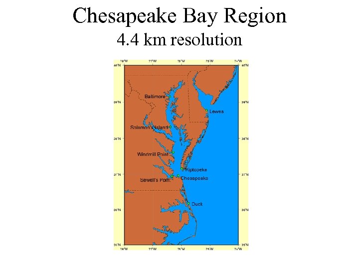
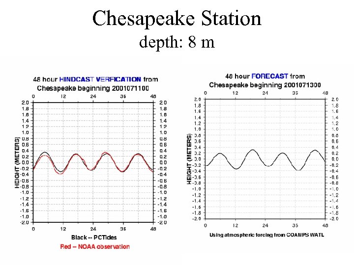
 Reliability • Both ADCIRC and PCTides generally produce sea level predictions that are within 10 cm and 30 minutes of observed values. • There are some areas of the world, such as off the U. S. West Coast, where results may be worse than quoted above due to reduced accuracy of the boundary conditions from the global tidal model. • The following images are from the PCTides OPTEST.
 Chesapeake Bay Region 4. 4 km resolution
 Chesapeake Station depth: 8 m
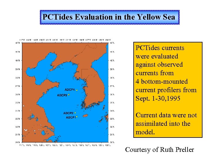 PCTides Evaluation in the Yellow Sea PCTides currents were evaluated against observed currents from 4 bottom-mounted current profilers from Sept. 1 -30, 1995 Current data were not assimilated into the model. Courtesy of Ruth Preller
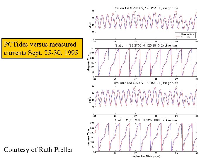 PCTides versus measured currents Sept. 25 -30, 1995 Courtesy of Ruth Preller
 References Blaine, C. A. , R. H. Preller, and A. P. Rivera, Tidal prediction using the Advanced Circulation Model (ADCIRC) and a relocatable PC-based system, Oceanography, 15 (1), 77 -87, 2002. Hubbert, G. D. , R. H. Preller, P. G. Posey, and S. N. Carroll, Software design description for the globally relocateable Navy time/atmosphere modeling system (PCTides), pp. 97, Naval Research Laboratory, Stennis Space Center, MS, 2001. Preller, R. H. , P. G. Posey, G. D. Hubbert, S. N. Carroll, and L. Orsi, User's manual for the globally relocatable Navy tide/atmosphere modeling system (PCTides), pp. 68, Naval Research Laboratory, Stennis Space Center, MS, 2001. Preller, R, P. Posey, G. Dawson, K. Miles, M. Escarra, J. Ganong (2002) http: //www 7320. nrlssc. navy. mil/pctides/
 Exercise • Get tidal height prediction for the same location using ADCIRC, PCTides, and GFMPL. Go to: http: //www. oc. nps. navy. mil/nom/PCTides/


