The World is Shriveling as it Shrinks Invited

The World is Shriveling as it Shrinks Invited Presentation Texas A & M College Station, TX, 26 October 2001 Waldo Tobler Professor Emeritus Geography Department University of California Santa Barbara, CA 93106 -4060 http: //www. geog. ucsb. edu/~tobler

Geographers know a lot about transportation The Von Thünen model is familiar to most

Agricultural patterns in the Von Thünen model with a modification due to river transportation

Some effects of a boundary on a trade area + Modified from A. Lösch, The Economics of Location

El Paso bank customers A. Lösch, The Economics of Location

What I hope to do in this talk is to give you some other ways of looking at the world. My interest in movement modeling is because most geographical change comes about because of movement. What is important is the movement of ideas, of people, money, energy, or material.

The often used phrase “The World is Shrinking” really refers to measurement in cost or time. 100 years ago the transportation cost for me to get here would have been prohibitive, and the travel time probably measured in weeks. The 80 days to travel around the world have been reduced to about 24 hours. So we all know that the world is shrinking. I hope to show you that this shrinking is very uneven and that the world is shriveling as well as shrinking.

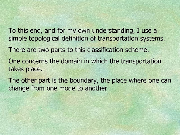
Transportation Systems

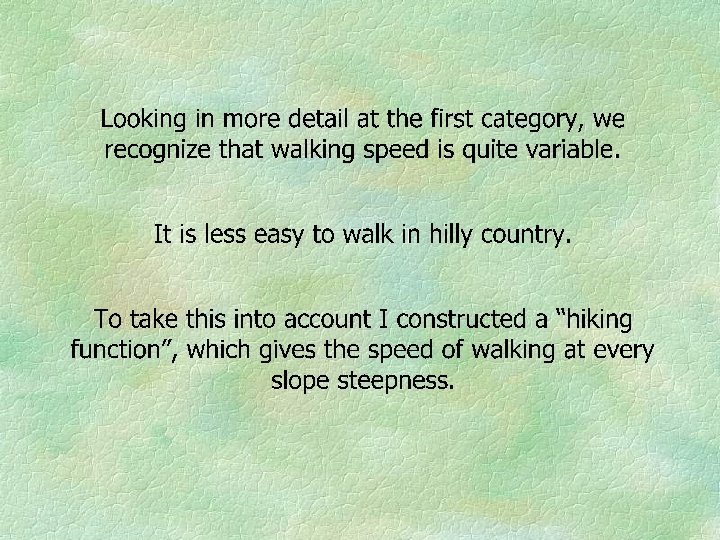
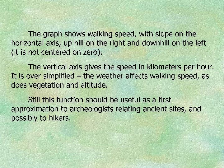
An Estimated Hiking Function

A simple topographic surface

Least time paths on the surface from the center

Isochrones - constant time contours about the center

Gradients added to produce polar coordinates about the center

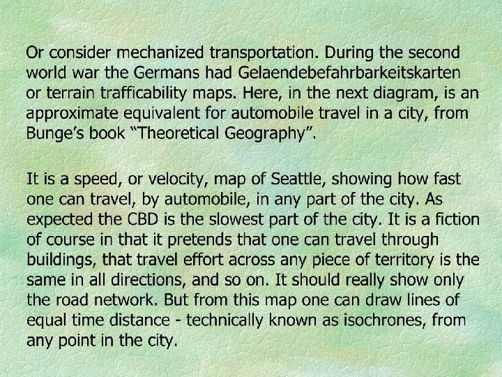
Travel Speed in Seattle In Miles per 5 minutes Measured by automobile driving time. This shows a scalar function, one value at each location. In reality it should be a tensor function, a different value in each direction at every location.

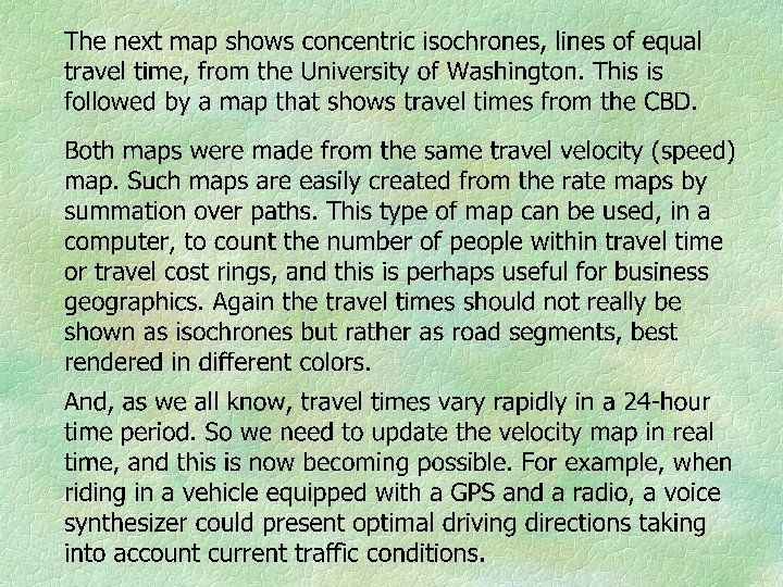
Peak Hour Travel Time from UW In Five Minute Intervals Draw orthogonal trajectories to the isolines. Think of these as the gradients to the contours. The two sets of curves form a system of curvilinear coordinates, known as polar geodesic coordinates. This coordinate system not only identifies locations but can be used analytically for metrical operations.

Five Minute Isochrones from CBD Travel time from Seattle’s central business district, in five minute intervals. Draw in the orthogonal trajectories, to turn the isolines into a system of polar coordinates. W. Bunge, 1966, Theoretical Geography, 2 nd ed. , Gleerup, Lund University

Time Distance from CBD Background Warped The travel times are now concentric circles. The geographic background has been warped to fit this. The orthogonals are now equally spaced straight lines (not drawn) radiating from the center to give the usual polar coordinates. W. Bunge, op. cit.

Travel Time from Berlin in Days Eckert, 1909

Travel Time from London In Hours

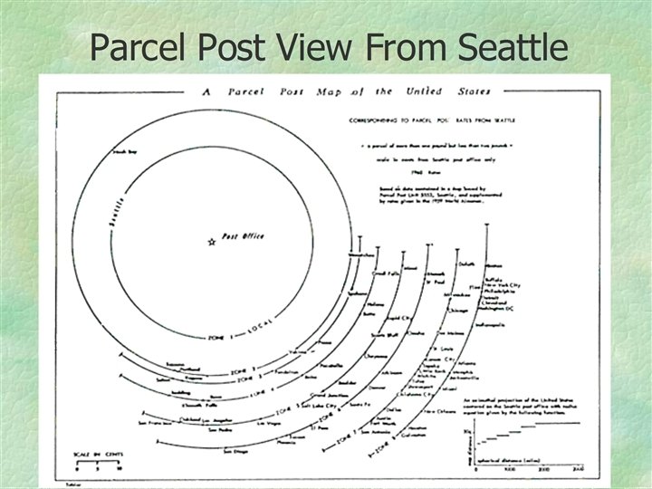
Check an airline rate book and you will find that Santa Barbara is closer in cost space to New York City than it is to Arcata in Northern California. Even worse, to fly from Santa Barbara to Columbus, Ohio, or to Milwaukee, Wisconsin, costs more than to fly to from Santa Barbara to New York City. In cost-space Columbus and Milwaukee are further from Santa Barbara than is New York City.

Thus the United States must again be turned inside out, in a very complicated way. Spend an hour or two with a rate table and you will find many such examples. Try to construct an air travel cost map centered on College Station, placing US and foreign cities at their scaled proper cost distance. It will be most instructive. There is not a monotonic relation between geographic distance in kilometers and geographic distance in monetary units. Thus I contend that the world is shriveling, with many places becoming relatively more isolated, and only a few becoming more connected.

Next is another, carefully done, example. It shows the one-hour vicinity of Liege, in Belgium. I say it is carefully done because the author recognizes several modes of transportation. It is only a single time slice, although travel schedules and frequencies were taken into account. An obvious question is “Can this type of diagram be made dynamic, in real time? ”

A One Hour Geographical Circle Liege 1958

Leipzig: The Six Hour Isochrone 1911

Now a little aside on geometry Distances determine geometry To calculate distances we use coordinates So here’s an example

x 1=1 y 1=1 1 2 3 x 2=7 y 2=6 4 5 6 7 8

Distance from (1, 1) to (7, 6) D = [(1 - 7)2 + (1 - 6)2]1/2 = [62 + 52]1/2 = [36 + 25]1/2 = 611/2 7. 8

x 1=1 y 1=1 1 2 3 x 2=7 y 2=6 4 5 6 7 8

Changing the name (coordinates) of a point does not alter the distance between them. But the rule whereby we calculate the distances does change. The next slide shows the same line in a new, different naming scheme (coordinate system).

x 1=1 y 1=1 1 2 x 2=4 y 2=6 3 4

Distance from (1, 1) to (4, 6) D = [(1 - 4)2 + (1 - 6)2]1/2 = [32 + 52]1/2 = 341/2 5. 8 which is wrong! But it can be fixed D = [4(1 -4)2 + (1 -6)2]1/2 = [4(32) + 52]1/2 = [36 + 25]1/2 7. 8 D 2=Wxdx 2 + dy 2

X 1=1 y 1=1 x 2=5 y 2=6

In these oblique coordinates The name of one point has again changed. What is the new rule to compute the distance?

Try the following D 2 = Wxdx 2 + Wxydxdy + Wyxdydx + Wydy 2 = Wxdx 2 + 2 Wxydxdy + Wydy 2 here Wxy = Wyx is related to the cosine of the angle between the axes. Wx and Wy are constants. Work out the details for yourself.

A more complicated example Curvilinear coordinates 4 3 2 1 1 2 3 4 5

With this new coordinate system the rule for the calculation of distances must again change . Needed now is a rule to be applied to a curvilinear coordinate system. Gauss invented such a rule in the early 1800’s. On surfaces that are not flat it is necessary to use such curvilinear coordinates and the Gaussian rule.

In the Gaussian metric formula d 12 = [(x 1 - x 2)2 + (y 1 - y 2)2]1/2 becomes dij 2 = Edu 2 + 2 Fdudv +Gdv 2 in modern notation ds 2 = gαβ duα duβ Written out in full this is, in two dimensions, ds 2 = g 11 dx 2 + g 12 dxdy + g 21 dydx+ g 22 dy 2 The coefficients are no longer constants. They are different in each curvilinear quadrangle. In polar coordinates: d 12 =[r 12 + r 22 - 2 r 1 r 2 cos(θ 1 - θ 2)]1/2 ds 2 = dr 2 + g 22 dθ 2

Some consequences applying to non-flat surfaces Circumference = 2 sin(r/√k) = 2 r - ( kr 3/3) + … Area = 2 (1 - cos(r/√k)) = r 2 - ( kr 4/12) + … The Gaussian curvature k is given, in polar geodesic coordinates, by k = -1/ (g 22)½dr 2

The relation between distance and curvature can be explained in more detail. As an example use distances on the earth.

Construct a table of distances between all places on the earth. Assume 2*107 places. The distance table contains n(n-1)/2 distances = 2*10 14 distances. Assume 200 distances per page for 1012 pages. At 6 grams/page this is 6*106 tons. Assume 6 tons per truck for 106 truckloads. Assume one truck every 5 seconds for 5*106 seconds, which is 2 months of day and night traffic. C. Misner, K. Thorne, J. Wheeler, 1973, Gravitation, Freeman, 306 -309.

Lots of trucks But the quantity of information can be reduced.

Use only the distance to nearby locations For each point record the distance to the nearest 100 points. Now there are only 2*109 distances. Or 107 pages of data, or 60 tons of paper. Needing only 10 truckloads, passing by in less than a minute.

Next assume that the surface is smooth and that the distance to points near another point can be approximated by the Euclidean distance formula. A triangulation can thus be established and distances to points further away can be calculated using the triangles. The approximation can be improved by taking more, and smaller, triangles.

A sample triangulation

Compute the angles in a triangle on the Euclidean assumption, using “small” triangles

Consider all triangles surrounding a vertex and lay them flat

In this way the curvature can be approximated at all locations. The curvature can also be calculated from the Gaussian coefficients gαβ So, instead of using a large number of distances use the Gaussian formula ds 2 = gαβ duα duβ

To use the Gaussian formula we need the three metrical coefficients, gij (i, j = 1, 2) at each of many geographical locations. But we might give these as functions of latitude and longitude, in terms of a power series or an expansion in spherical harmonics, with a modest number say 100, of adjustable coefficients. Then the information about the geometry is caught up in these three hundred coefficients, a single page printout. Goodbye to any truck! Considering the earth as a sphere the coefficients would all be constant, and therefore we need only one constant.

Now try using travel times, or costs, instead of spherical kilometers to calculate the curvature. The result could be quite interesting. Some people have tried to fit mathematical functions to the geographic travel time or cost spaces. They generally use either Minkowski or Manhattan metrics. Riemannian or Finsler geometry seems to me to offer more promise.

Geographers have long used travel time or cost maps. Most travel time/cost maps are centered on one location.

US Road Distances Map Student drawing

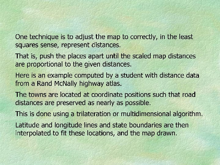
The road distance map is distorted relative to the normal map. From theory of cartography we know that map distortion can be measured using Tissot’s strain tensor, and this can serve as a measure of the change introduced into the United States by the road system. Are there policy implications?

Measure Distances Along the “Road”

Alternately, raise the places into the air so that the Euclidean distance in three space gives the correct distance, in road distance space, in time distance space, or in cost distance space. That is, use least squares to go from a representation in X, Y space go to a representation in X, Y, Z space. Then, from the point representation in 3 -D, interpolate to get a "transportation surface".

Interpolated Transportation Surface Measure distances as arc length on the surface

Europe Now

The next figure shows the warping that will be introduced by the high speed network, as measured in travel time space. The scale is given in hours, rather than kilometers and shows what Europe will look like when the high speed network is completed. Observe that France is furthest along, and therefore the most shrunken. The assumption has been made that one can interpolate from the rail network to the entire continent. Again, from cartographic theory, we know that not only are conventional distances distorted on this map but that areas and angles are also distorted, and we can compute by how much. Thus we can measure the distorting effect of transportation, using Tissot’s theorem.

Europe After The Proposed TGV System Spiekerman & Wegener

A profoundly more realistic example, by Alain L’Hostis, is from France. Best viewed in color at http: //www. inrets. fr/traces/equipe/lhostis. htm This is where I got the term shriveling. Maybe it should be wrinkling. The map is in perspective, but shows three transportation systems simultaneously, using travel time as the metric. First, on top and with the shortest connections, is the high speed rail system (TGV). Then below this is the freeway system, in blue. Distances are to be measured along the blue lines, over hill and dale. Below these two is the ordinary road network. Measure along the lighter lines. This is a 3 D version of the resistor diagram shown earlier.

The TGV Warps Space By A. L’Hostis

One can get to any place in France using a combination of the three modes of transport. From this diagram one can see how a new disease might diffuse from a rural location and quickly get transmitted to Paris, or how an idea could spread from Paris to other parts of the country before getting to remote “backwaters”. Slightly unrealistic is the assumption that going from the TGV train to the freeway takes no time, air travel has been omitted, and that travel time is the same in both directions. Admittedly measuring on this map would be difficult but this diagram is nevertheless a most marvelous invention, conceptually and graphically! With GIS technology one might drape the conventional map of France on top of this transportation surface. A dynamic version would pulsate.

Bunge suggested constrained balloons. Fix strings to wellconnected places (NYC, LAX, etc) then inflate the balloon. The less well connected places will bulge out. (Bunge, personal communication, ca, 1960)

We are not finished An important property of geographic distance measures has been overlooked

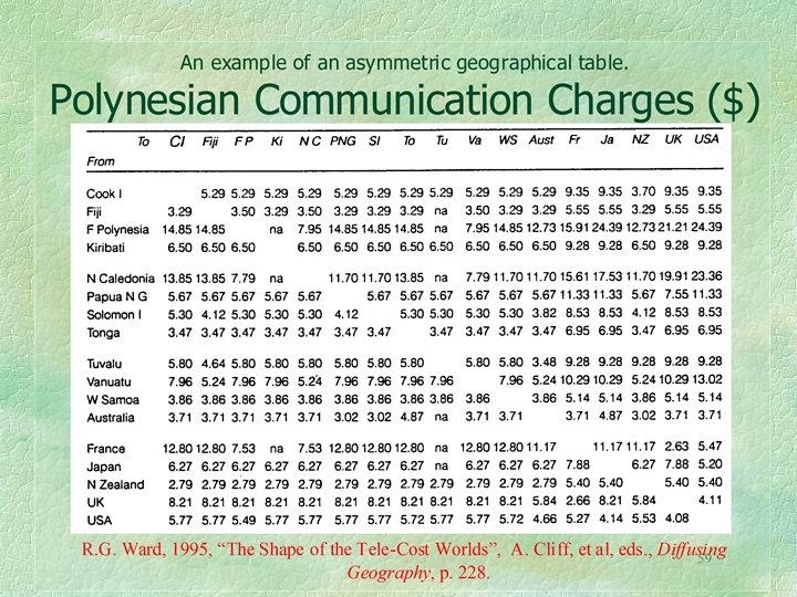
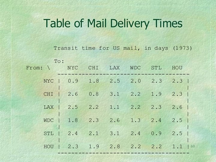
Here is another very small example of a geographic table. It shows mail delivery times, in days, between a few cities in the United States. The cities are New York, Chicago, Los Angeles, Washington D. C. , St. Louis, and Houston. There are many examples of such asymmetric tables, especially when considering costs. Any such table can be decomposed into symmetric and skew symmetric parts, each of which contributes to the total variance.

A Map of Wind Computed from Mail Delivery Times

From Wind to Pressure Field An interesting property of vector fields, as on the foregoing map, is that they may be inverted. If you think of a vector field as having been derived from the topography of some surface this assertion is that the topography can be calculated when only the slope is known. At least up to a constant of integration (the absolute elevation) and if the data are curl free. In the particular instance here, this says that the barometric pressure could be estimated from the mail delivery times.

What I am asserting is that one approach to the asymmetry problem is to add a vector field to the distances. This makes movement in particular directions easier or more difficult. Such a vector field might be applied to simulations of the spread of ideas, and so on. There are several possible mathematical implementations to this idea. See: W. Tobler, “Spatial Interaction Patterns”. Journal of Environmental Systems, 6, 4 (1976 -77): 271 -301.

Finally, in contemplating relations between places on the earth I hope that I have convinced you that it is often not the geodetic distance that is most important but rather the time or cost which must be overcome. Some places are now closer but others are relatively further away. This is why I assert that The earth is shriveling as it shrinks.

Citations W. Bunge, 1966, Theoretical geography, 2 nd ed. , Greelup, Lund. R. Love, & Morris, J. , 1979, “Modeling Inter-City Road Distances by Mathematical Functions”, Operational Research Quarterly, 23: 61 -71. C. Gauss, 1910, General Investigations on curved surfaces (1827), Princton University Press, Princeton. F. Dussart, 1959, “Les courbes isochrones de la ville de Liege pour 19581959”, Bull. Soc. Belge d’Etudes Geog. , XXVIII(1): 59 -68. C. Misner, K. Thorne, J. Wheeler, 1973, Gravitation, Freeman, San Francisco. J. Riedel, 1911, “Neue Studien Űber Isochronenkarten”, Pet. Geog. Mitt. , LVII(1): 281 -284. K. Spiekermann, Wegener, M. , 1994, “The Shrinking Continent”, Environment & Planning, B, 21: 651 -673. E. Zaustinsky, 1959, Spaces with non-symmetric distance, Memoir 34, American Mathematical Society, 91 pp.