

355ea3d4e18580a39b01d4e51431cd0b.ppt
- Количество слайдов: 74
 The Use of Geometrical and Physical Models in Quantitative Medical Image Analysis James S. Duncan, Ph. D. Departments of Diagnostic Radiology and Electrical Engineering Yale University
 Collaborators • Segmentation: -Larry Staib -Amit Chakraborty -Isil Bozma -Xiaolan Zeng • Cardiac Deformation: - Xenios Papademetris - Pengcheng Shi -Albert Sinusas, M. D. -Todd Constable • Brain Shift Compensation: - Oskar Skrinjar - Dennis Spencer, M. D.
 Outline I. Overview of Problem Areas - will focus on 3 heart/brain problems - types of 3 D/4 D Image Datasets II. Using Geometrically- Based Models - segmentation - motion tracking - neuroanatomical measurement III. Using Biomechanical Models - cardiac deformation analysis - brain shift compensation in neurosurgery
 Outline I. Overview of Problem Areas - will focus on 3 heart/brain problems - types of 3 D/4 D Image Datasets II. Using Geometrically- Based Models - segmentation - motion tracking - neuroanatomical measurement III. Using Biomechanical Models - cardiac deformation analysis - brain shift compensation in neurosurgery
 Active Research Areas in Medical Image Analysis • Image Distortion Correction • Quantitative Measurement of Anatomy/ Physiology • Quantitative Characterization of Disease • Data/ Information Handling/Fusion • Modeling/ prediction of Function/Disease • Improved Visualization of All of Above • Image- Guided Intervention/Surgery
 We’ll Look at Several of These Issues from the Viewpoint of Three Examples: a. ) Characterization of Cardiac Function from Noninvasive 4 D Imaging b. ) Study of Neuroanatomical Structure from MRI c. ) Brain Shift Compensation in Image Guided Neurosurgery
. Recovery of Cardiac Deformation (Problem Statement)") a. ). Recovery of Cardiac Deformation (Problem Statement)
a. ). Recovery of Cardiac Deformation (Problem Statement)
 The Left Ventricle ED ES 2 D Motion Analysis X-ray Ventriculography
 15 Minutes RV LAD 40 Minutes LV 3 Hours Nonischemic 6 Hours Occluded Vascular Bed (area at risk) Infarct
 4 D Cardiac Image Datasets
 Canine Experiment") Transmyocardial Revascularization (TMR) Canine Experiment
Transmyocardial Revascularization (TMR) Canine Experiment
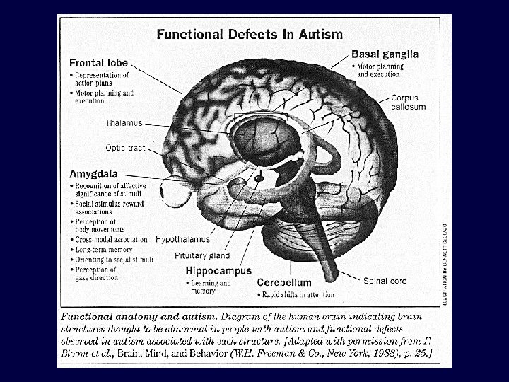
 Measurement of Neuroanatomical Structure (Problem Statement)") b. ) Measurement of Neuroanatomical Structure (Problem Statement)
b. ) Measurement of Neuroanatomical Structure (Problem Statement)
 Example Neuroanatomical Structures of Interest 3 D MRI data Parcellated cortex
 Brain Shift Compensation in Image-Guided Neurosurgery (Problem Statement)") c. ) Brain Shift Compensation in Image-Guided Neurosurgery (Problem Statement)
c. ) Brain Shift Compensation in Image-Guided Neurosurgery (Problem Statement)
 Neurosurgical Issues Related to Brain Shift • Navigation via Image-Guided Stereotactic System is Difficult/ Inaccurate: - perceived vs. actual position of structures (especially below the surface) off by many mm. - especially problematic for placing depth electrodes during epilepsy surgery • in Epilepsy Surgery: Implanted Electrode Arrays (used to gather confirmatory functional information) further deform brain: - now difficult to relate to preop estimates of seizure location (from SPECT/PET) and/or cognitive activity (f. MRI) • Tumor localization (especially below the surface) difficult in Image -Guided system both pre- and post- resection
 Forms of Brain Deformation • Typical Post-Craniotomy Shift for different gray/CSF surface positions: 0. 75 mm to 7. 5 mm (per D. Hill, et al, CVRMed 97) • Average Brain Shift Post(Tumor/ Hematoma) Resection, in Surrounding Region: 9. 5 mm/7. 9 mm (per Bucholz, et al. , CVRMed 97)
 All 3 Examples Involve the Same Basic Algorithmic Steps • Segment Structural Boundaries from 3 D/4 D image datasets: - Invoke Model for Context • Recover Quantitative Information (size/ motion/deformation) about Heart or Brain: - Models Guide this Process • Visualize Results (most helpful to relate to raw image data) Each Step Utilizes Geometrical or Biomechanical Models !
 Outline I. Overview of Problem Areas - will focus on 3 heart/brain problems - types of 3 D/4 D Image Datasets II. Using Geometrically- Based Models - segmentation - motion tracking - neuroanatomical measurement III. Using Biomechanical Models - cardiac deformation analysis - brain shift compensation in neurosurgery
 Geometrical Models: Segmentation
 Segmentation: Why is it useful in Medical Image analysis ? • identify anatomical structure/ landmarks/ROI’s for : • measurement of anatomy and function • to help register and then compare images • visualization of structure and function • group spatially-related functional activity
") Segmentation: What’s typically used ? • Manual outlining of structure (problems: reproducibility, labor intense) • thresholding gray level histograms (no sense of spatial connectivity) • seed simple region growing algorithms that fill within isocontours (poor accuracy on real data) • feature clustering of multiecho MR images to get tissue classes (no spatial connectivity)
Segmentation: What’s typically used ? • Manual outlining of structure (problems: reproducibility, labor intense) • thresholding gray level histograms (no sense of spatial connectivity) • seed simple region growing algorithms that fill within isocontours (poor accuracy on real data) • feature clustering of multiecho MR images to get tissue classes (no spatial connectivity)
 Our Take on Deformable Model- based approaches to Segmentation • Have looked generally at one structure at a time • Desire to utilize BOTH bounding structure and region homogeneity constraints • Feel that there are two general classes of problems in the brain: 1. ) “find something that roughly looks like this global shape” (e. g. the LV, many subcortical structures) 2. ) “locate the most locally-coherent structure according to these constraints” (e. g. the outer cortex)
 ;") Related Work from Other Groups • Shape Priors: Cootes and Taylor (IPMI 93) ; Grenander/ Miller (atlases/templates- 1991) ; Vemuri, et al. (Med. IA 97) • Integrated Methods: 1. ) Region grow w/ edges. Pavlidis and Liow (PAMI 91); Zhu and Yuille (ICCV 95) ; Ahuja (PAMI 96) 2. ) level sets - Tek and Kimia (ICCV 95) • Segment/ Measure Cortical Gray Matter: Macdonald and Evans (SPIE 95) ; Teo and Sapiro (TMI 97) ; Xu and Prince (MICCAI 98) ; Davatzikos (TMI 95 - ribbons) • Also see Review of Deformable Models by Mc. Inerney and Terzopolous, Medical Image Analysis, Vol. 1 No. 2, 1996.
Related Work from Other Groups • Shape Priors: Cootes and Taylor (IPMI 93) ; Grenander/ Miller (atlases/templates- 1991) ; Vemuri, et al. (Med. IA 97) • Integrated Methods: 1. ) Region grow w/ edges. Pavlidis and Liow (PAMI 91); Zhu and Yuille (ICCV 95) ; Ahuja (PAMI 96) 2. ) level sets - Tek and Kimia (ICCV 95) • Segment/ Measure Cortical Gray Matter: Macdonald and Evans (SPIE 95) ; Teo and Sapiro (TMI 97) ; Xu and Prince (MICCAI 98) ; Davatzikos (TMI 95 - ribbons) • Also see Review of Deformable Models by Mc. Inerney and Terzopolous, Medical Image Analysis, Vol. 1 No. 2, 1996.
") Parametrically Deformable Boundary Finding (posed as MAP Estimation)
Parametrically Deformable Boundary Finding (posed as MAP Estimation)
 The Influence of Prior Shape Orig image Region segment. Intialization/ Shape prior Integrated (region-segment. - Gradient -based boundary finder- NO prior (Left Thalamus) boundary finderinfluenced) Objective: NO prior locate Left Thalamus Gradient-based boundary finder WITH shape prior Integrated boundary finder WITH shape prior
 3 D LV Segmentation Using Prior Shape Model Short Axis Long Axes
") Integrated Segmentation via Game Theory Region-Based segmentation Image P 1* = X (classified pixels) P 2 Boundary Finding P 2* = p (boundary parameters)
Integrated Segmentation via Game Theory Region-Based segmentation Image P 1* = X (classified pixels) P 2 Boundary Finding P 2* = p (boundary parameters)
 Game-Theoretic Integration- Results Test image: SNR =0. 67 Black= initialization White = gradientbased result Black= intialization White = result with gametheoretic integration Black = gradient-based White = game -theoretic
 Subcortical Structure Segmentation Integrated Algorithm results Manual Expert Tracing Left Caudate Nucleus Right Thalamus
 Interactive Seeding and Correction
 Coupled Surfaces: Image Feature Extraction • MR bias field correction performed using simple nonlinear map • local operator is used to derived the likelihood of a voxel lying on the boundary of tissues A and B Orig image gradient gray/white CSF/gray
) 1 0 p(q*) h(d) 0 min max |d| d: distance") Coupled Surfaces Propagation g(p(q*)) 1 0 p(q*) h(d) 0 min max |d| d: distance between the two bounding surfaces A=white matter, B= gray matter, C= CSF
Coupled Surfaces Propagation g(p(q*)) 1 0 p(q*) h(d) 0 min max |d| d: distance between the two bounding surfaces A=white matter, B= gray matter, C= CSF
 Coupled Surface Segmentation Results Initialization Gray/CSF surface Gray/White surface
 Coupled Surfaces vs. Single Surface Segmentation 2 single 3 D surfaces Note: coupled surfaces approach prevents inner surface from collapsing into CSF Note: the coupled surfaces approach prevents the outer surface from penetrating non-brain tissue 3 D coupled surfaces (Sagittal cuts through 3 D result)
 Geometrical Models: Cardiac Motion Tracking
 Cardiac Motion Tracking: Related Work from Other Groups • MR Tagging: Young and Axel, 1993 ; Park, Metaxas, and Axel, 1995 ; Denney and Prince, 1994. • MR Phase Contrast Velocities: Pelc, Herfkens and L. Pelc, 1992; Meyer, Constable, Sinusas and Duncan, 1995. • Biomechanical Model- based Tracking efforts: Guccione, Mc. Culloch and Waldman, 1991; Park and Metaxas, 1996.
 Finding Principal Curvatures • for any surface patch: curves C of max and min curvature = principal curvatures • directions on plane tangent to normal plane are principal directions Principal directions along LV endocardial surface (from DSR)
 Curvatures are Relatively Stable From Time Frame to Time Frame e. g. , note Bending Energies: (White = less bending away from flat plane, Green= more bending) From cine-MRI from DSR
 u v t 2 Shape Based Matching t 1 t 2 t 1 u d 0 d v Smoothed Displacement Vectors
 ED to ES Motion Trajectories MRI CT
 MRI Validation w/ Markers
 CT Validation
 Initial Evaluation of Shape-Based Displacement: Comparison to Post Mortem/ SPECT Shape- Tracked Displacements classified by path length white = normal, blue = short, yellow/red =long Post- mortem TTC staining SPECT -derived perfusion blue = injury zone, red = normal white = normal, blue = short, yellow/red =long (n=5 canine studies) MRI/shape(in vivo) Estimated infarct area 796 +/- 124 Post mortem 783 +/- 131 correlation r=. 968
 Geometrical Models: Measurement of Neuroanatomical Structure
 Right Frontal") Cortical Thickness Measurements on N = 30 normal male controls: Region (lobe) Right Frontal Left Post. Right Post 3. 40(. 43) Thickness Left Frontal 3. 25 (. 42) 3. 06(. 41) 3. 00(. 40) (mm) (+/- SD) Two examples: brain 1: (a and b), brain 2: (c) Note marked thinning in postcentral gyrus and prim/sec visual cortices 1 3 5 (thickness in mm)
Cortical Thickness Measurements on N = 30 normal male controls: Region (lobe) Right Frontal Left Post. Right Post 3. 40(. 43) Thickness Left Frontal 3. 25 (. 42) 3. 06(. 41) 3. 00(. 40) (mm) (+/- SD) Two examples: brain 1: (a and b), brain 2: (c) Note marked thinning in postcentral gyrus and prim/sec visual cortices 1 3 5 (thickness in mm)
 Shape Index Map cup saddle cap
 Extract sulcal bottom and top curves Initialize surface: piecewise") Sulcal Surface Finding (Cont. ) Extract sulcal bottom and top curves Initialize surface: piecewise linear mesh Surface deformation to medial axis (using distance function) Brain Parcellation
Sulcal Surface Finding (Cont. ) Extract sulcal bottom and top curves Initialize surface: piecewise linear mesh Surface deformation to medial axis (using distance function) Brain Parcellation
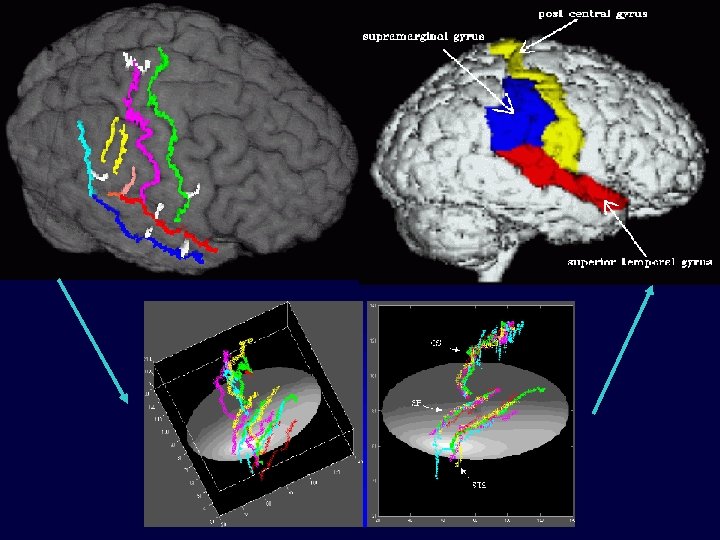
 Detected Sulcal Ribbons Right Central Sulcus Right Frontal Superior Left Central Sulcus Left Frontal Superior
 interhemispheric fissure ; central sulcus") Robust Point Matching of Sulcal Patterns (5 patient datasets) interhemispheric fissure ; central sulcus ; sylvian fissure ; superior temporal sulcus
Robust Point Matching of Sulcal Patterns (5 patient datasets) interhemispheric fissure ; central sulcus ; sylvian fissure ; superior temporal sulcus
 Outline I. Overview of Problem Areas - will focus on 3 heart/brain problems - types of 3 D/4 D Image Datasets II. Using Geometrically- Based Models - segmentation - motion tracking - neuroanatomical measurement III. Using Biomechanical Models - cardiac deformation analysis - brain shift compensation in neurosurgery
 Biomechanical Models: Quantifying Left Ventricular Deformation
 Recovery and Quantification of LV Strain • GOAL: Recover Dense 3 D Strains for Deforming Left Ventricle • DATA: Shape-based (or MR tag-based) Displacements, sometimes Phase Contrast MRI- based velocities • APPROACH: - Biomechanical models of the LV used to guide recovery and reporting of strain information - Tradeoffs as to when to use image-derived data and when to invoke model are made via data confidence measures.
 in") LV Material Model • Defined as an internal strain energy function = W(e) in general, where e = the local strain tensor • For our model, we assume linear elasticity, thus W(e) = et C e, where C = the constitutive relation (material properties) for the LV • Different forms of C are: I. ) An Isotropic, Linear Elastic Model: Where E = Young’s modulus (~75 Kpascal) n = Poisson’s ration (about. 5 ~ incompressible
LV Material Model • Defined as an internal strain energy function = W(e) in general, where e = the local strain tensor • For our model, we assume linear elasticity, thus W(e) = et C e, where C = the constitutive relation (material properties) for the LV • Different forms of C are: I. ) An Isotropic, Linear Elastic Model: Where E = Young’s modulus (~75 Kpascal) n = Poisson’s ration (about. 5 ~ incompressible
 II. ) An Anisotropic, Linear Elastic Model: Where Ef") LV Material Model (cont. ) II. ) An Anisotropic, Linear Elastic Model: Where Ef = fiber stiffness Ep = cross fiber stiffness (Ef ~4 Ep) nfp, npp = corresponding Poisson’s ratios (~0. 4) Gf ~ Ef / [2(1+ nfp)] (shear modulus across fibers)
LV Material Model (cont. ) II. ) An Anisotropic, Linear Elastic Model: Where Ef = fiber stiffness Ep = cross fiber stiffness (Ef ~4 Ep) nfp, npp = corresponding Poisson’s ratios (~0. 4) Gf ~ Ef / [2(1+ nfp)] (shear modulus across fibers)
 Assume small deformation (infinitesimal strain) between frames") Solution via Finite Element Method 1. ) Assume small deformation (infinitesimal strain) between frames (<5%), thus e = Bu, where: B = displacement-strain Jacobian (implicit are FEM interpolating functions) u = displacement vector at each node n of element mesh representing the LV. 2. ) The same interpolating functions can be used to describe a continuous 3 D displacement function u(x, y, z) from concatenated set of all nodes = U. a 3. ) In our computation, we seek to find u(x, y, z) that minimizes the potential energy: internal/strain energy (model) external energy (data)
Solution via Finite Element Method 1. ) Assume small deformation (infinitesimal strain) between frames (<5%), thus e = Bu, where: B = displacement-strain Jacobian (implicit are FEM interpolating functions) u = displacement vector at each node n of element mesh representing the LV. 2. ) The same interpolating functions can be used to describe a continuous 3 D displacement function u(x, y, z) from concatenated set of all nodes = U. a 3. ) In our computation, we seek to find u(x, y, z) that minimizes the potential energy: internal/strain energy (model) external energy (data)
 4. ) the above minimization problem can be") Solution via Finite Element Method (cont) 4. ) the above minimization problem can be rewritten in terms of finding the discrete U where: 5. ) given: W(U) = Ut. KU , K a function of C (material matrix), B (Jacobian) and assuming V(U) = (Ue-U)t A (Ue-U), where Ue are image-based displacements and A is the confidence matrix 6. ) we can differentiate the equation in 4. ) to get:
Solution via Finite Element Method (cont) 4. ) the above minimization problem can be rewritten in terms of finding the discrete U where: 5. ) given: W(U) = Ut. KU , K a function of C (material matrix), B (Jacobian) and assuming V(U) = (Ue-U)t A (Ue-U), where Ue are image-based displacements and A is the confidence matrix 6. ) we can differentiate the equation in 4. ) to get:
 dynamic terms can be added to 6.") Solution via FEM: Adding Dynamics 7. ) dynamic terms can be added to 6. ), as can image- derived velocity information: where now: Ad and Av are the displacement and velocity data confidence matrices M is the mass matrix- a function of B (FEM-approximated displacementstrain Jacobian and assumed mass density r C is the damping matrix, a small fraction of M Solve using Newmark integration Mag fx fy fz MR phase contrast velocity images
Solution via FEM: Adding Dynamics 7. ) dynamic terms can be added to 6. ), as can image- derived velocity information: where now: Ad and Av are the displacement and velocity data confidence matrices M is the mass matrix- a function of B (FEM-approximated displacementstrain Jacobian and assumed mass density r C is the damping matrix, a small fraction of M Solve using Newmark integration Mag fx fy fz MR phase contrast velocity images
 Normal Canine Heart 1 Hour Post- LAD Occlusion") Radial Strain from MRI (Shape-Tracking) Normal Canine Heart 1 Hour Post- LAD Occlusion
Radial Strain from MRI (Shape-Tracking) Normal Canine Heart 1 Hour Post- LAD Occlusion
 Circumferential Strain") Radial Strains Derived from cine- MRI (Canine study: post occlusion) Circumferential Strain
Radial Strains Derived from cine- MRI (Canine study: post occlusion) Circumferential Strain
 Circumferential Strain") Radial Strains Derived from 3 D Echo (Canine study: post occlusion) Circumferential Strain
Radial Strains Derived from 3 D Echo (Canine study: post occlusion) Circumferential Strain
 Biomechanical Models: Brain Shift Compensation for Image- Guided Neurosurgery
 …") Previous Efforts in Brain Shift Estimation • Bucholz, et al. , (CVRMed 1997) … used Intraoperative ultrasound and 2 D spring -based mechanical model (looked at a variety of structure pre/post op on n=23 pts) … (2 D datasets only) • Hill, Fitzpatrick, et al. , (CVRMed 1997) … measured brain shifts relative to skull on 5 patients using ACUSTAR I (fiducial-based) surgical navigation system. . . (measurements only) • Edwards, Hill, Little, Hawkes, (IPMI 1997)… 3 component (rigid, deformable, fluid), physically-motivated, energy-based model; used landmark-like data. . . (2 Dran in 2 -3 hours on SPARC 20) • Kyriacou, Davatzikos, (MICCAI 1998) … 2 D Continuum model via FEMaimed at larger deformations (e. g. tumors)… (so far 2 D- primarily simulation) • Miga, Paulsen, et al. , (MICCAI 1998)… 3 D Continuum/FEM model tested/validated on Porcine brains… (nice effort- primarily forward modeling)
Previous Efforts in Brain Shift Estimation • Bucholz, et al. , (CVRMed 1997) … used Intraoperative ultrasound and 2 D spring -based mechanical model (looked at a variety of structure pre/post op on n=23 pts) … (2 D datasets only) • Hill, Fitzpatrick, et al. , (CVRMed 1997) … measured brain shifts relative to skull on 5 patients using ACUSTAR I (fiducial-based) surgical navigation system. . . (measurements only) • Edwards, Hill, Little, Hawkes, (IPMI 1997)… 3 component (rigid, deformable, fluid), physically-motivated, energy-based model; used landmark-like data. . . (2 Dran in 2 -3 hours on SPARC 20) • Kyriacou, Davatzikos, (MICCAI 1998) … 2 D Continuum model via FEMaimed at larger deformations (e. g. tumors)… (so far 2 D- primarily simulation) • Miga, Paulsen, et al. , (MICCAI 1998)… 3 D Continuum/FEM model tested/validated on Porcine brains… (nice effort- primarily forward modeling)
 System Block Diagram Segment Acquired Pre-op 3 D MRI/ locate skin markers Develop Mesh for Entire Brain Identify skin markers in OR via OMI system LMSE Registration *Touch 6 points on Brain with OMI arm Initialize Model with Estimated kd and ks at each node Pre- operative Estimate Model Parameters From N=10 training Sets Model Repeat every 10 minutes (x 5) Deform Brain Mesh (* initial strategy) Intra-operative Update Image Texture Maps/ Surfaces
 Static Biomechanical Modelling • Due to relatively small order of local brain deformation, we choose a linear elastic model with infinitesimal (<5%) strain • From standard formulations (e. g. minimum potential energy), for this model, with f = total force acting on body, u = displacement for any and all points : or Ku = f K 1 K 2 u = f where K 1 is due to geometry and K 2 due to material (stiffness) parameters • We choose a nodal geometry, yielding spring-like interactions between the nodes: i j
 Nodes in Model Mesh Approximately 2088 node points/ volumetric brain model
 Biomechanical Modelling: Adding Dynamics In general, from Newton’s 2 nd Law: For our linear elastic nodal model, the dynamics of each node i reduce to: j fij i j j mg node i node j ks nij
 : Compute") Brain-Skull Interaction • Now handled using a “contact” algorithm (from numerical analysis) : Compute new node position from model update skull Node returned Gray/CSF boundary Does node enter skull ? no Node moves freely Leave current node position yes Return node to previous position
Brain-Skull Interaction • Now handled using a “contact” algorithm (from numerical analysis) : Compute new node position from model update skull Node returned Gray/CSF boundary Does node enter skull ? no Node moves freely Leave current node position yes Return node to previous position
 Cranial Opening and Points Recorded on Brain Surface 12 cm 3 c m 12 cm
 Point- Driven Brain Shift Compensatinon Without Compensation With Model- Based Compensation
 Point- Based 3 D Brain Model Deformation
 Movement/error in mm Preliminary Results: Model + 2 Marked Points vs. Other 4 Points 4 Mean brain surface movement 3 2 Mean error (4 pts predicted from 2 pts) 1 0 0 10 20 30 40 Time from opening of Dura 50
") Alternative Intra-operative Data Acquisition Strategies • Dual visible light cameras (recover surface via stereo) • Structured light (surface only) • ultrasound probe (2 D/3 D) • Intra-operative MRI • Portable CT scanner (e. g. Philips)
Alternative Intra-operative Data Acquisition Strategies • Dual visible light cameras (recover surface via stereo) • Structured light (surface only) • ultrasound probe (2 D/3 D) • Intra-operative MRI • Portable CT scanner (e. g. Philips)