The Simple Linear Regression Model Specification and Estimation

The Simple Linear Regression Model: Specification and Estimation Chapter 2

Chapter 2: The Simple Regression Model 2. 1 An Economic Model 2. 2 An Econometric Model 2. 3 Estimating the Regression Parameters 2. 4 Assessing the Least Squares Estimators 2. 5 The Gauss-Markov Theorem 2. 6 The Probability Distributions of the Least Squares Estimators 2. 7 Estimating the Variance of the Error Term Principles of Econometrics, 3 rd Edition Slide 2 -2

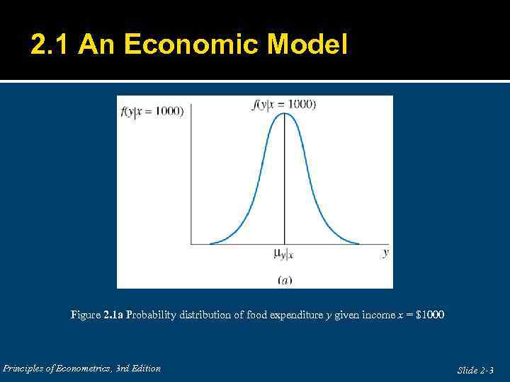2. 1 An Economic Model Figure 2. 1 a Probability distribution of food expenditure y given income x = $1000 Principles of Econometrics, 3 rd Edition Slide 2 -3

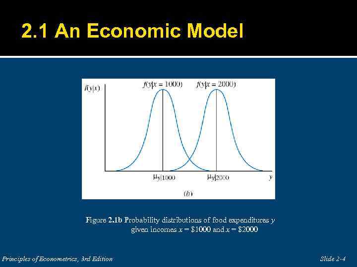2. 1 An Economic Model Figure 2. 1 b Probability distributions of food expenditures y given incomes x = $1000 and x = $2000 Principles of Econometrics, 3 rd Edition Slide 2 -4

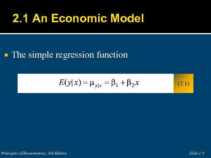2. 1 An Economic Model The simple regression function (2. 1) Principles of Econometrics, 3 rd Edition Slide 2 -5

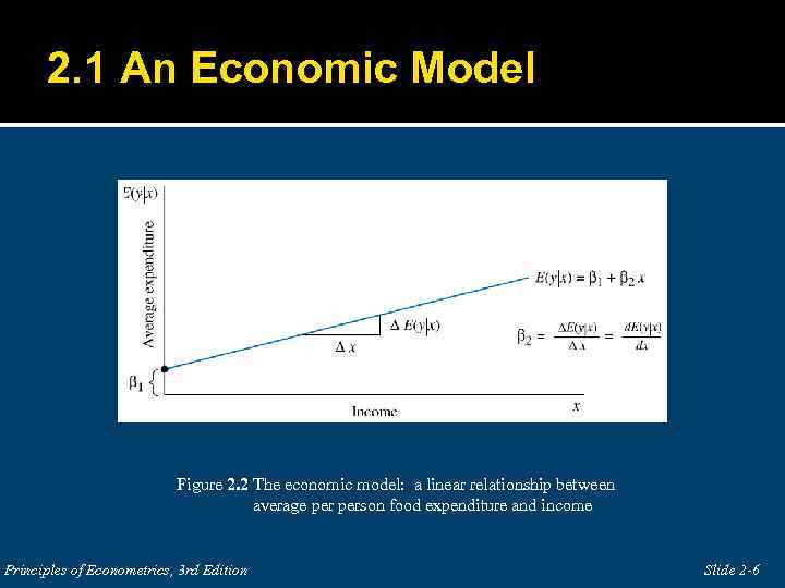2. 1 An Economic Model Figure 2. 2 The economic model: a linear relationship between average person food expenditure and income Principles of Econometrics, 3 rd Edition Slide 2 -6

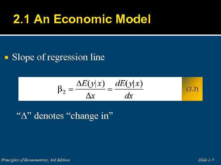2. 1 An Economic Model Slope of regression line (2. 2) “Δ” denotes “change in” Principles of Econometrics, 3 rd Edition Slide 2 -7

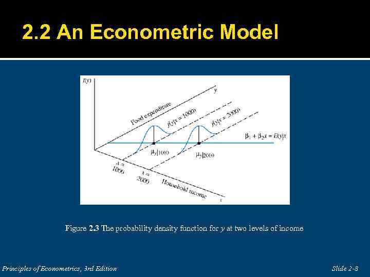2. 2 An Econometric Model Figure 2. 3 The probability density function for y at two levels of income Principles of Econometrics, 3 rd Edition Slide 2 -8

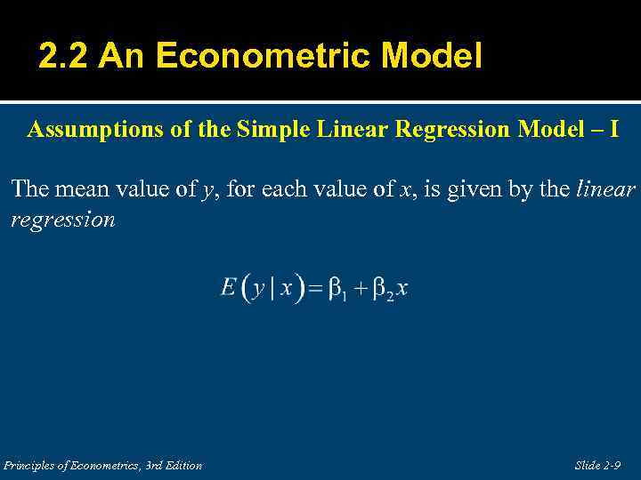2. 2 An Econometric Model Assumptions of the Simple Linear Regression Model – I The mean value of y, for each value of x, is given by the linear regression Principles of Econometrics, 3 rd Edition Slide 2 -9

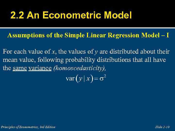2. 2 An Econometric Model Assumptions of the Simple Linear Regression Model – I For each value of x, the values of y are distributed about their mean value, following probability distributions that all have the same variance (homoscedasticity), Principles of Econometrics, 3 rd Edition Slide 2 -10

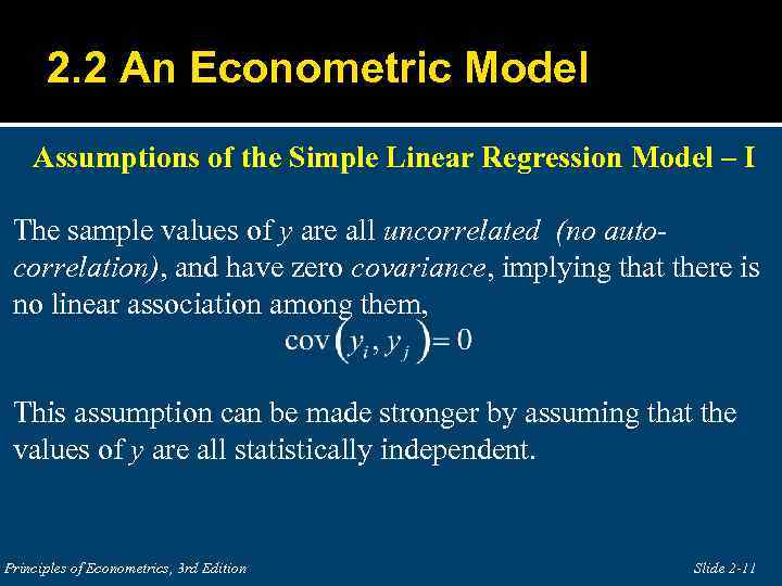2. 2 An Econometric Model Assumptions of the Simple Linear Regression Model – I The sample values of y are all uncorrelated (no autocorrelation), and have zero covariance, implying that there is no linear association among them, This assumption can be made stronger by assuming that the values of y are all statistically independent. Principles of Econometrics, 3 rd Edition Slide 2 -11

2. 2 An Econometric Model Assumptions of the Simple Linear Regression Model – I The variable x is not random, and must take at least two different values. Principles of Econometrics, 3 rd Edition Slide 2 -12

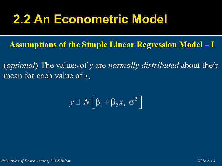2. 2 An Econometric Model Assumptions of the Simple Linear Regression Model – I (optional) The values of y are normally distributed about their mean for each value of x, Principles of Econometrics, 3 rd Edition Slide 2 -13

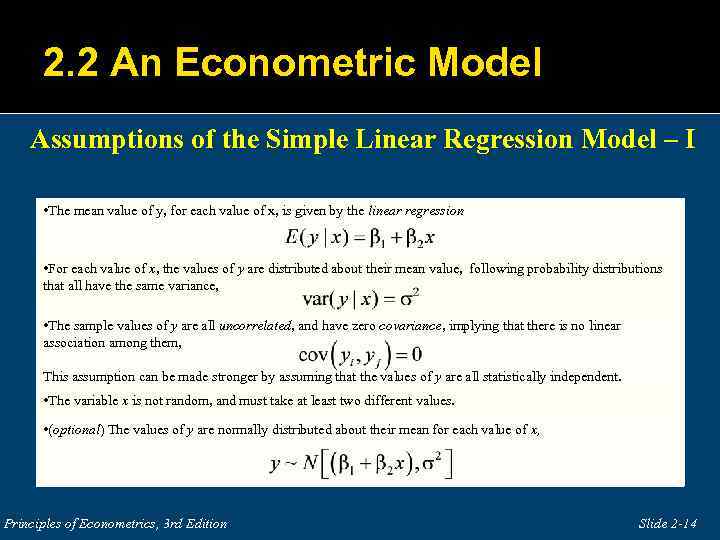2. 2 An Econometric Model Assumptions of the Simple Linear Regression Model – I • The mean value of y, for each value of x, is given by the linear regression • For each value of x, the values of y are distributed about their mean value, following probability distributions that all have the same variance, • The sample values of y are all uncorrelated, and have zero covariance, implying that there is no linear association among them, This assumption can be made stronger by assuming that the values of y are all statistically independent. • The variable x is not random, and must take at least two different values. • (optional) The values of y are normally distributed about their mean for each value of x, Principles of Econometrics, 3 rd Edition Slide 2 -14

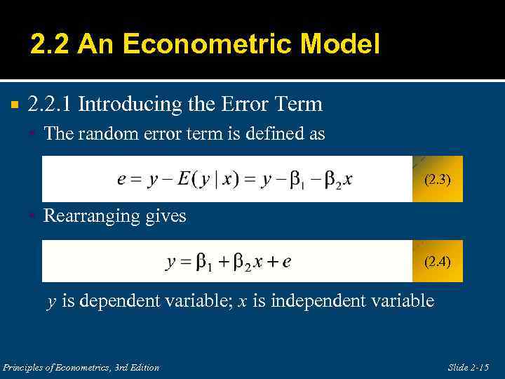2. 2 An Econometric Model 2. 2. 1 Introducing the Error Term The random error term is defined as (2. 3) Rearranging gives (2. 4) y is dependent variable; x is independent variable Principles of Econometrics, 3 rd Edition Slide 2 -15

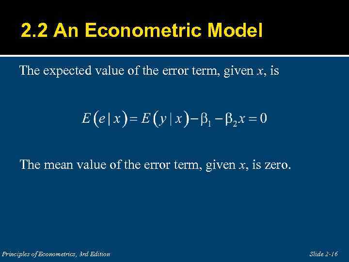2. 2 An Econometric Model The expected value of the error term, given x, is The mean value of the error term, given x, is zero. Principles of Econometrics, 3 rd Edition Slide 2 -16

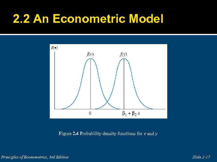2. 2 An Econometric Model Figure 2. 4 Probability density functions for e and y Principles of Econometrics, 3 rd Edition Slide 2 -17

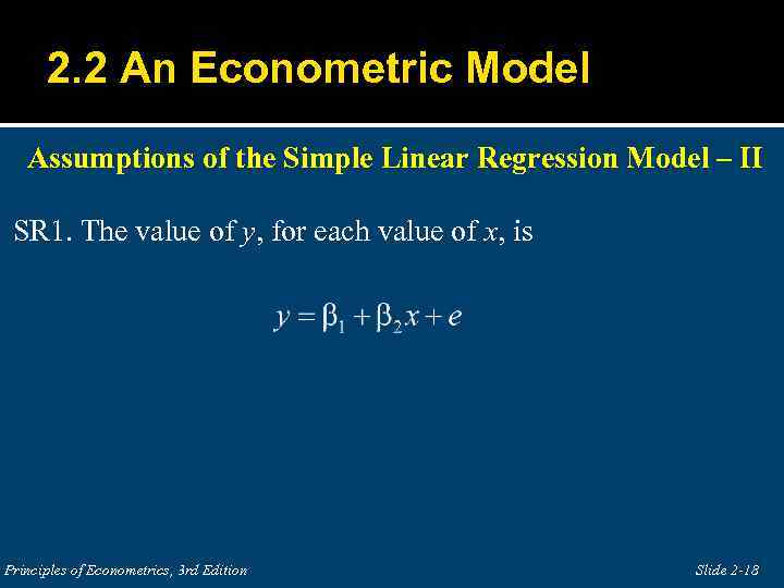2. 2 An Econometric Model Assumptions of the Simple Linear Regression Model – II SR 1. The value of y, for each value of x, is Principles of Econometrics, 3 rd Edition Slide 2 -18

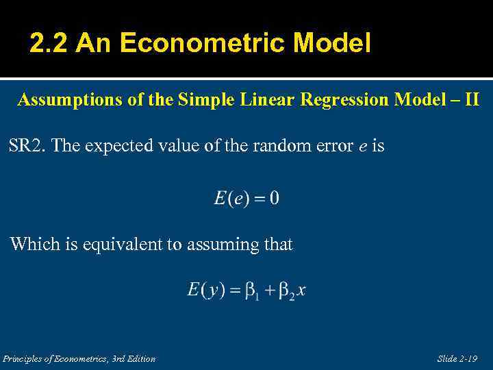2. 2 An Econometric Model Assumptions of the Simple Linear Regression Model – II SR 2. The expected value of the random error e is Which is equivalent to assuming that Principles of Econometrics, 3 rd Edition Slide 2 -19

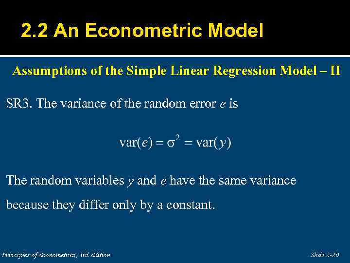2. 2 An Econometric Model Assumptions of the Simple Linear Regression Model – II SR 3. The variance of the random error e is The random variables y and e have the same variance because they differ only by a constant. Principles of Econometrics, 3 rd Edition Slide 2 -20

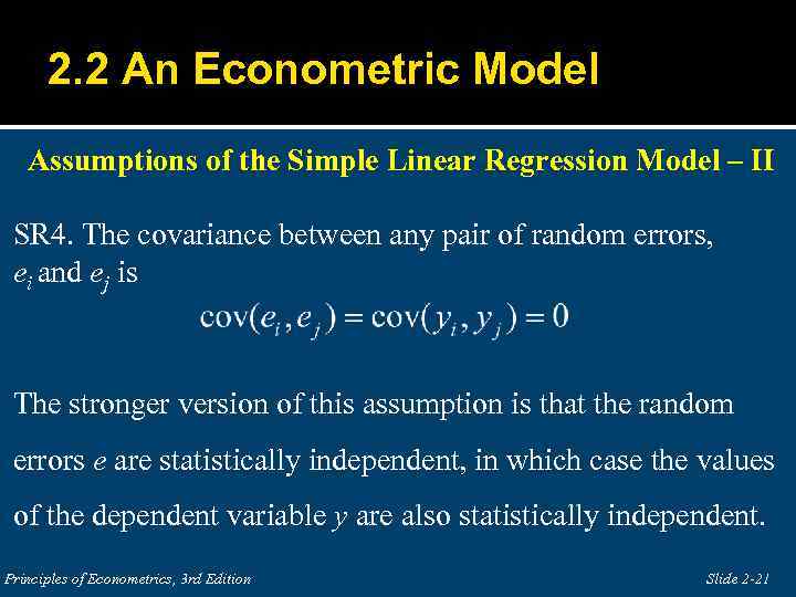2. 2 An Econometric Model Assumptions of the Simple Linear Regression Model – II SR 4. The covariance between any pair of random errors, ei and ej is The stronger version of this assumption is that the random errors e are statistically independent, in which case the values of the dependent variable y are also statistically independent. Principles of Econometrics, 3 rd Edition Slide 2 -21

2. 2 An Econometric Model Assumptions of the Simple Linear Regression Model – II SR 5. The variable x is not random, and must take at least two different values. Principles of Econometrics, 3 rd Edition Slide 2 -22

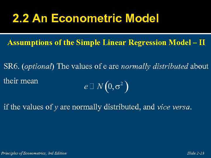2. 2 An Econometric Model Assumptions of the Simple Linear Regression Model – II SR 6. (optional) The values of e are normally distributed about their mean if the values of y are normally distributed, and vice versa. Principles of Econometrics, 3 rd Edition Slide 2 -23

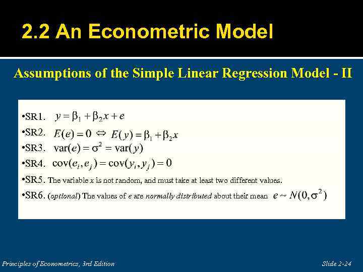2. 2 An Econometric Model Assumptions of the Simple Linear Regression Model - II • SR 1. • SR 2. • SR 3. • SR 4. • SR 5. The variable x is not random, and must take at least two different values. • SR 6. (optional) The values of e are normally distributed about their mean Principles of Econometrics, 3 rd Edition Slide 2 -24

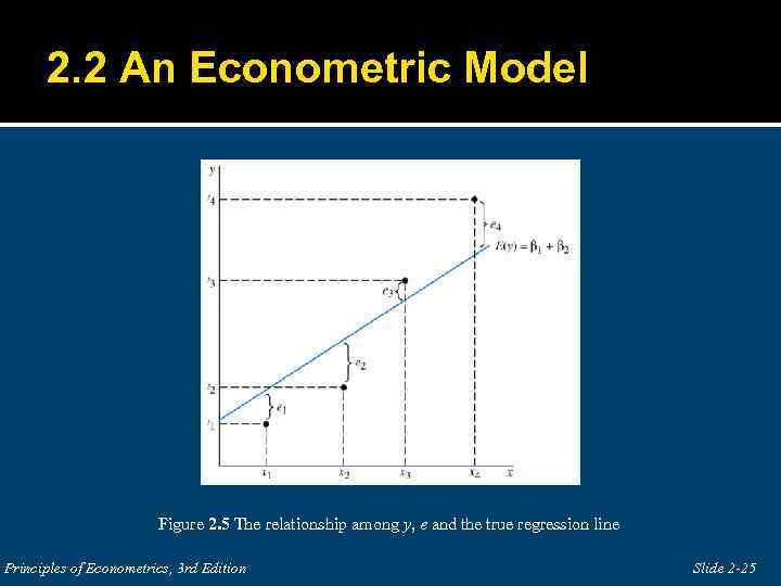2. 2 An Econometric Model Figure 2. 5 The relationship among y, e and the true regression line Principles of Econometrics, 3 rd Edition Slide 2 -25

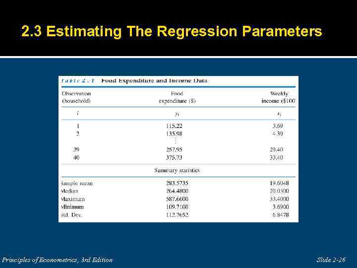2. 3 Estimating The Regression Parameters Principles of Econometrics, 3 rd Edition Slide 2 -26

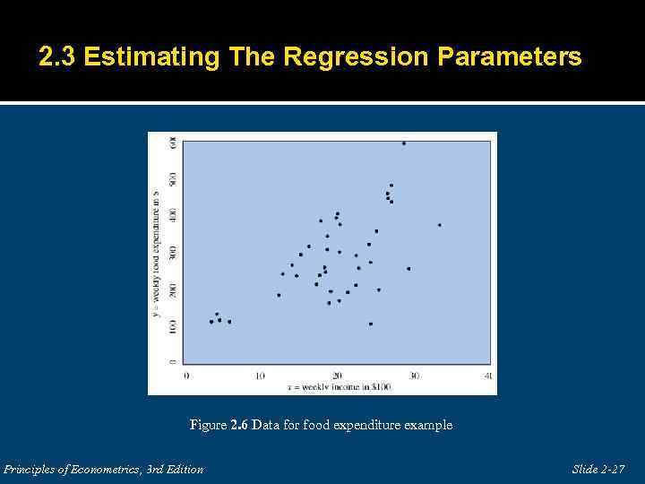2. 3 Estimating The Regression Parameters Figure 2. 6 Data for food expenditure example Principles of Econometrics, 3 rd Edition Slide 2 -27

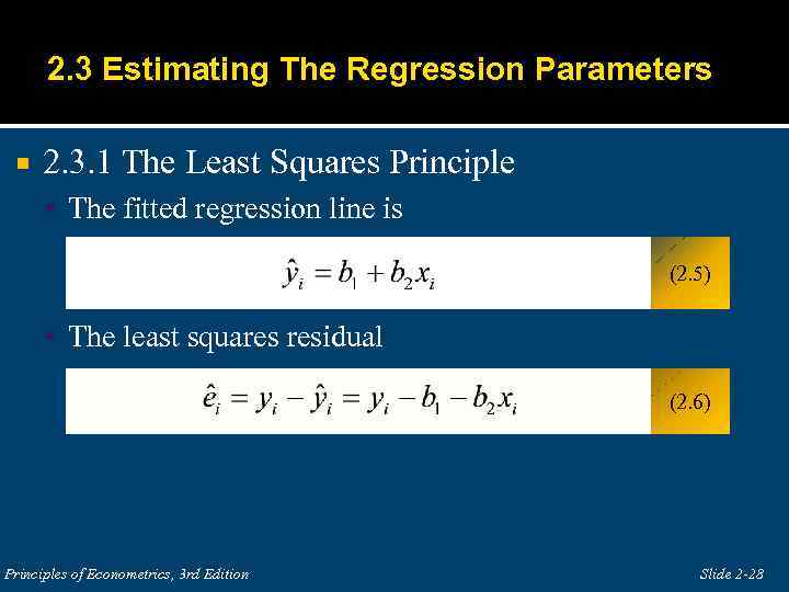2. 3 Estimating The Regression Parameters 2. 3. 1 The Least Squares Principle The fitted regression line is (2. 5) The least squares residual (2. 6) Principles of Econometrics, 3 rd Edition Slide 2 -28

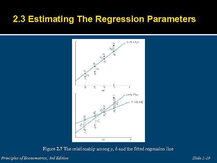2. 3 Estimating The Regression Parameters Figure 2. 7 The relationship among y, ê and the fitted regression line Principles of Econometrics, 3 rd Edition Slide 2 -29

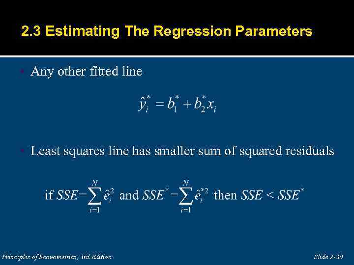2. 3 Estimating The Regression Parameters Any other fitted line Least squares line has smaller sum of squared residuals Principles of Econometrics, 3 rd Edition Slide 2 -30

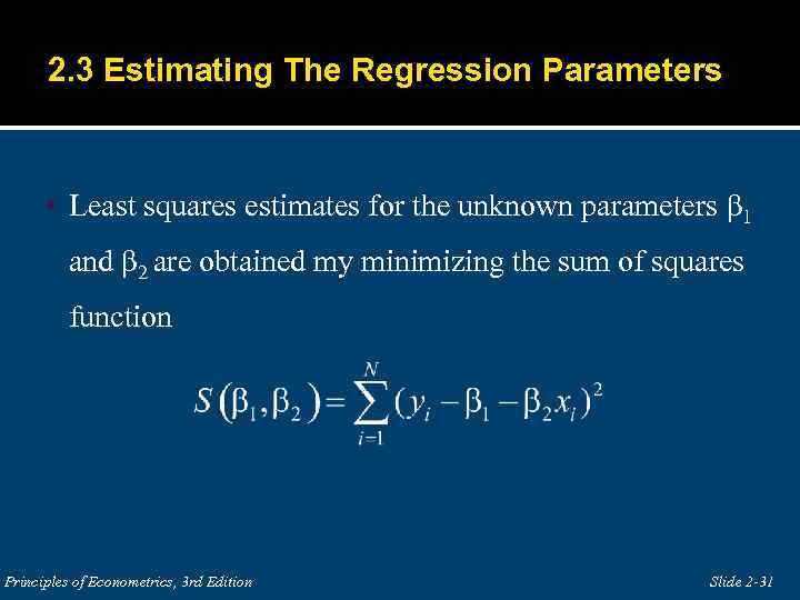2. 3 Estimating The Regression Parameters Least squares estimates for the unknown parameters β 1 and β 2 are obtained my minimizing the sum of squares function Principles of Econometrics, 3 rd Edition Slide 2 -31

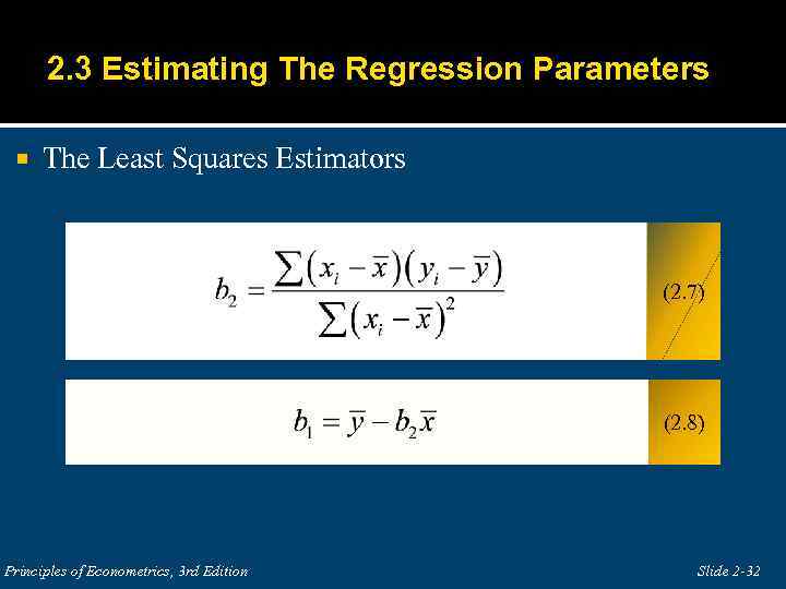2. 3 Estimating The Regression Parameters The Least Squares Estimators (2. 7) (2. 8) Principles of Econometrics, 3 rd Edition Slide 2 -32

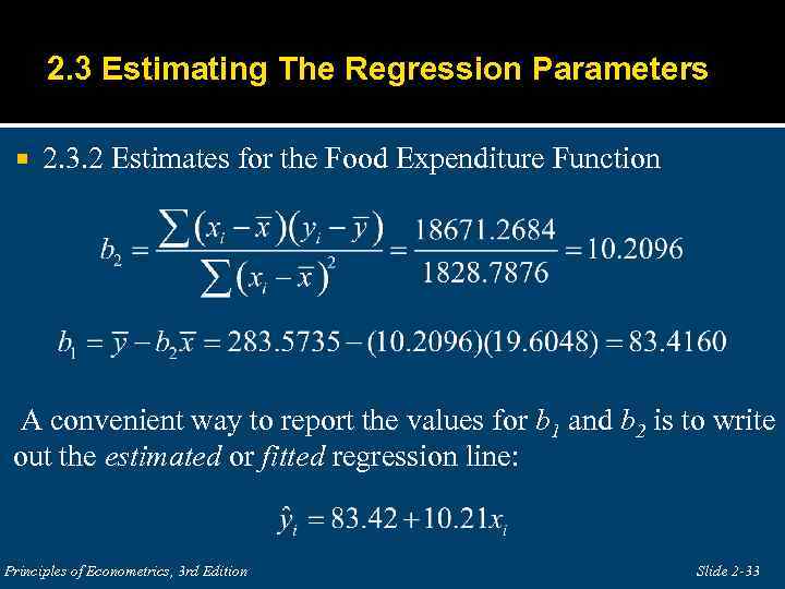2. 3 Estimating The Regression Parameters 2. 3. 2 Estimates for the Food Expenditure Function A convenient way to report the values for b 1 and b 2 is to write out the estimated or fitted regression line: Principles of Econometrics, 3 rd Edition Slide 2 -33

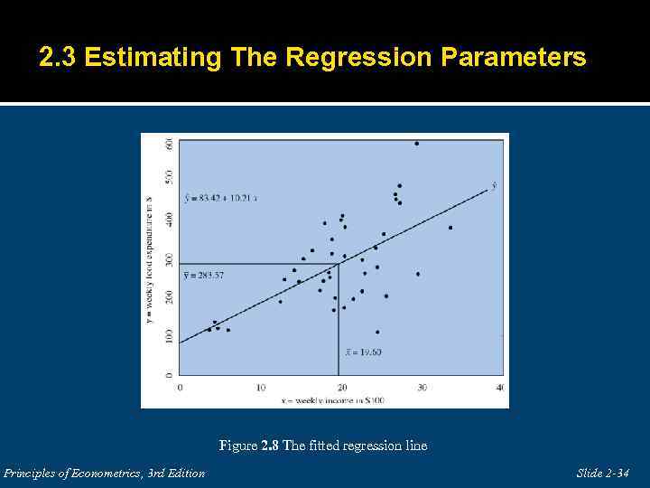2. 3 Estimating The Regression Parameters Figure 2. 8 The fitted regression line Principles of Econometrics, 3 rd Edition Slide 2 -34

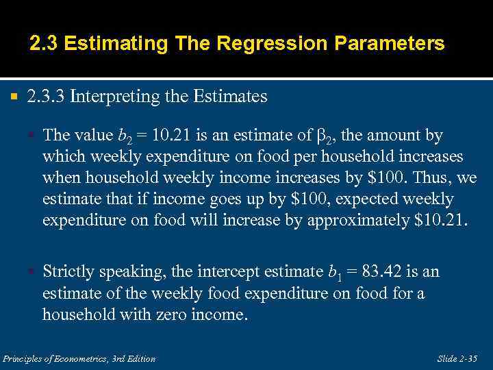2. 3 Estimating The Regression Parameters 2. 3. 3 Interpreting the Estimates The value b 2 = 10. 21 is an estimate of 2, the amount by which weekly expenditure on food per household increases when household weekly income increases by $100. Thus, we estimate that if income goes up by $100, expected weekly expenditure on food will increase by approximately $10. 21. Strictly speaking, the intercept estimate b 1 = 83. 42 is an estimate of the weekly food expenditure on food for a household with zero income. Principles of Econometrics, 3 rd Edition Slide 2 -35

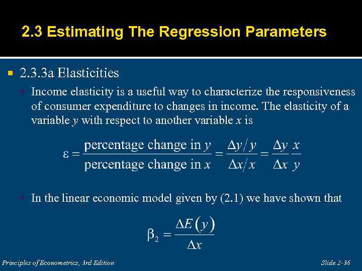2. 3 Estimating The Regression Parameters 2. 3. 3 a Elasticities Income elasticity is a useful way to characterize the responsiveness of consumer expenditure to changes in income. The elasticity of a variable y with respect to another variable x is In the linear economic model given by (2. 1) we have shown that Principles of Econometrics, 3 rd Edition Slide 2 -36

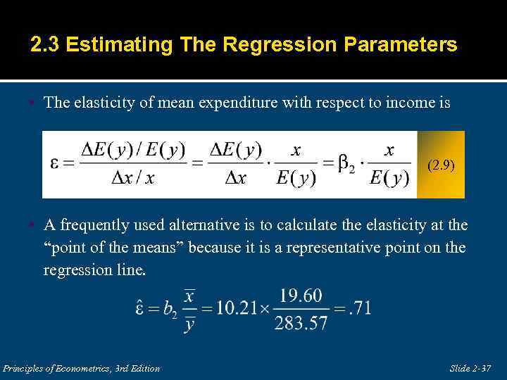2. 3 Estimating The Regression Parameters The elasticity of mean expenditure with respect to income is (2. 9) A frequently used alternative is to calculate the elasticity at the “point of the means” because it is a representative point on the regression line. Principles of Econometrics, 3 rd Edition Slide 2 -37

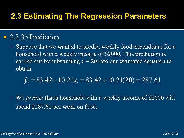2. 3 Estimating The Regression Parameters 2. 3. 3 b Prediction Suppose that we wanted to predict weekly food expenditure for a household with a weekly income of $2000. This prediction is carried out by substituting x = 20 into our estimated equation to obtain We predict that a household with a weekly income of $2000 will spend $287. 61 per week on food. Principles of Econometrics, 3 rd Edition Slide 2 -38

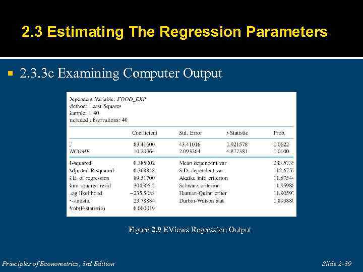2. 3 Estimating The Regression Parameters 2. 3. 3 c Examining Computer Output Figure 2. 9 EViews Regression Output Principles of Econometrics, 3 rd Edition Slide 2 -39

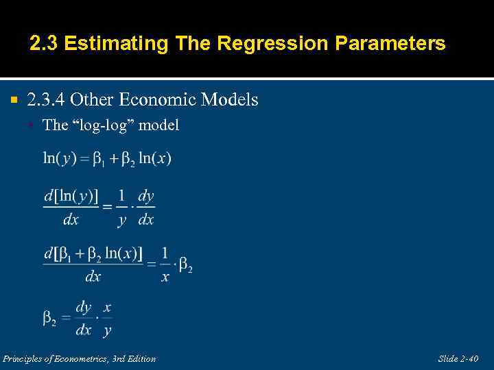2. 3 Estimating The Regression Parameters 2. 3. 4 Other Economic Models The “log-log” model Principles of Econometrics, 3 rd Edition Slide 2 -40

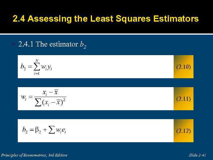2. 4 Assessing the Least Squares Estimators 2. 4. 1 The estimator b 2 (2. 10) (2. 11) (2. 12) Principles of Econometrics, 3 rd Edition Slide 2 -41

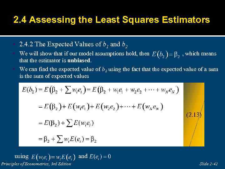2. 4 Assessing the Least Squares Estimators 2. 4. 2 The Expected Values of b 1 and b 2 We will show that if our model assumptions hold, then , which means that the estimator is unbiased. We can find the expected value of b 2 using the fact that the expected value of a sum is the sum of expected values (2. 13) using and Principles of Econometrics, 3 rd Edition Slide 2 -42

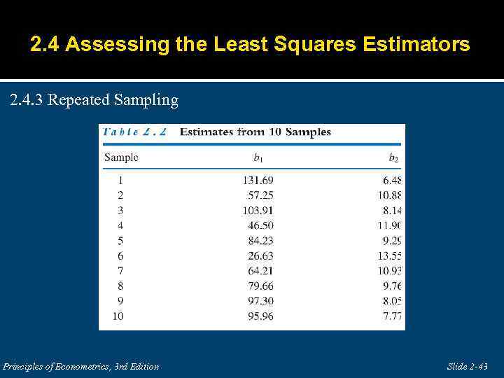2. 4 Assessing the Least Squares Estimators 2. 4. 3 Repeated Sampling Principles of Econometrics, 3 rd Edition Slide 2 -43

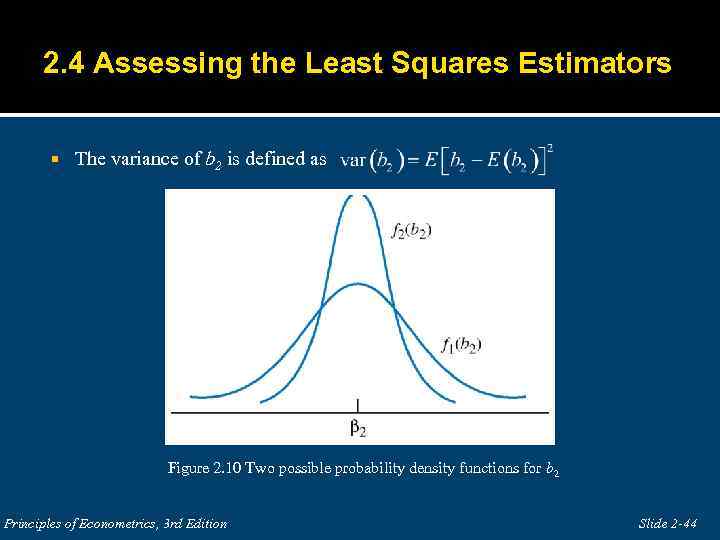2. 4 Assessing the Least Squares Estimators The variance of b 2 is defined as Figure 2. 10 Two possible probability density functions for b 2 Principles of Econometrics, 3 rd Edition Slide 2 -44

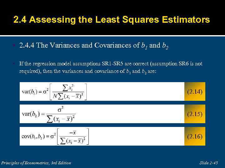2. 4 Assessing the Least Squares Estimators 2. 4. 4 The Variances and Covariances of b 1 and b 2 If the regression model assumptions SR 1 -SR 5 are correct (assumption SR 6 is not required), then the variances and covariance of b 1 and b 2 are: (2. 14) (2. 15) (2. 16) Principles of Econometrics, 3 rd Edition Slide 2 -45

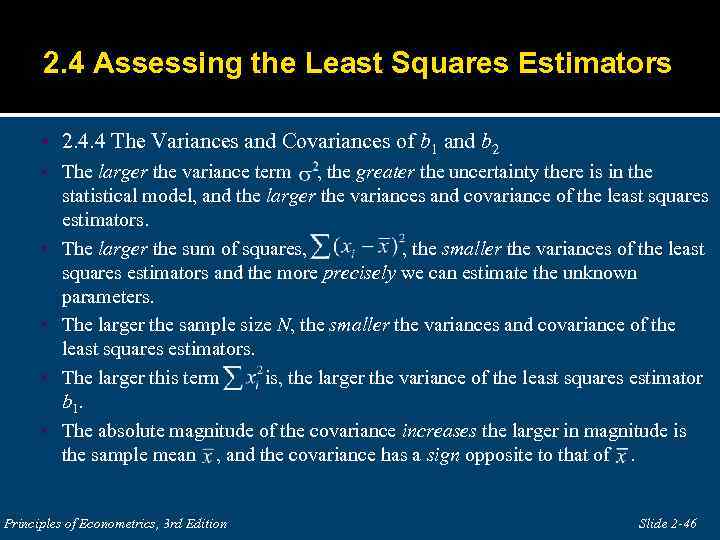2. 4 Assessing the Least Squares Estimators 2. 4. 4 The Variances and Covariances of b 1 and b 2 The larger the variance term , the greater the uncertainty there is in the statistical model, and the larger the variances and covariance of the least squares estimators. The larger the sum of squares, , the smaller the variances of the least squares estimators and the more precisely we can estimate the unknown parameters. The larger the sample size N, the smaller the variances and covariance of the least squares estimators. The larger this term is, the larger the variance of the least squares estimator b 1. The absolute magnitude of the covariance increases the larger in magnitude is the sample mean , and the covariance has a sign opposite to that of . of Econometrics, 3 rd Edition Principles Slide 2 -46

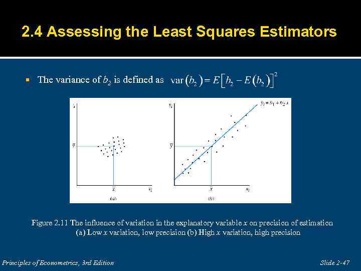2. 4 Assessing the Least Squares Estimators The variance of b 2 is defined as Figure 2. 11 The influence of variation in the explanatory variable x on precision of estimation (a) Low x variation, low precision (b) High x variation, high precision Principles of Econometrics, 3 rd Edition Slide 2 -47

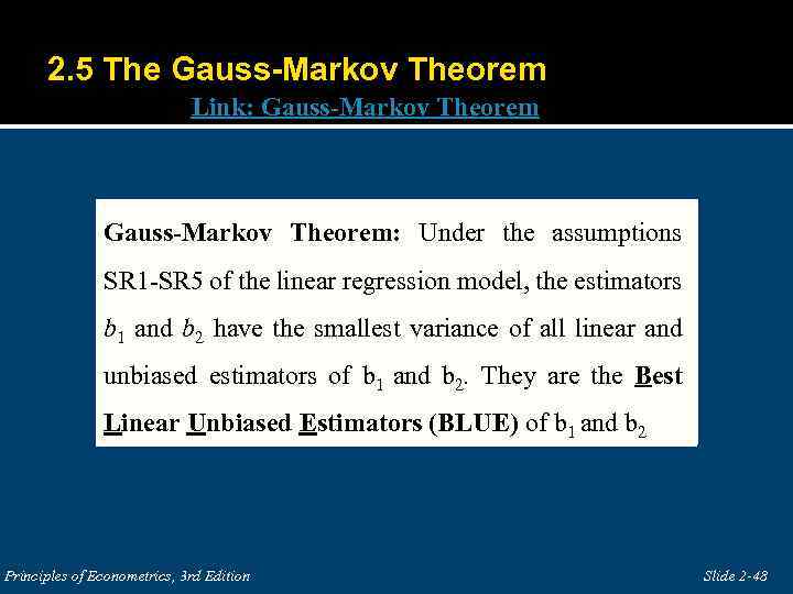2. 5 The Gauss-Markov Theorem Link: Gauss-Markov Theorem: Under the assumptions SR 1 -SR 5 of the linear regression model, the estimators b 1 and b 2 have the smallest variance of all linear and unbiased estimators of b 1 and b 2. They are the Best Linear Unbiased Estimators (BLUE) of b 1 and b 2 Principles of Econometrics, 3 rd Edition Slide 2 -48

2. 5 The Gauss-Markov Theorem 1. The estimators b 1 and b 2 are “best” when compared to similar estimators, those which are linear and unbiased. Theorem does not say that b 1 and b 2 are the best of all possible estimators. 2. The estimators b 1 and b 2 are best within their class because they have the minimum variance. When comparing two linear and unbiased estimators, we always want to use the one with the smaller variance, since that estimation rule gives us the higher probability of obtaining an estimate that is close to the true parameter value. 3. In order for the Gauss-Markov Theorem to hold, assumptions SR 1 -SR 5 must be true. If any of these assumptions are not true, then b 1 and b 2 are not the best linear unbiased estimators of β 1 and β 2. Principles of Econometrics, 3 rd Edition Slide 2 -49

2. 5 The Gauss-Markov Theorem 4. The Gauss-Markov Theorem does not depend on the assumption of normality (assumption SR 6). 5. In the simple linear regression model, if we want to use a linear and unbiased estimator, then we have to do no more searching. The estimators b 1 and b 2 are the ones to use. This explains why we are studying these estimators and why they are so widely used in research, not only in economics but in all social and physical sciences as well. 6. The Gauss-Markov theorem applies to the least squares estimators. It does not apply to the least squares estimates from a single sample. (In other words, you can have a weird sample. ) Principles of Econometrics, 3 rd Edition Slide 2 -50

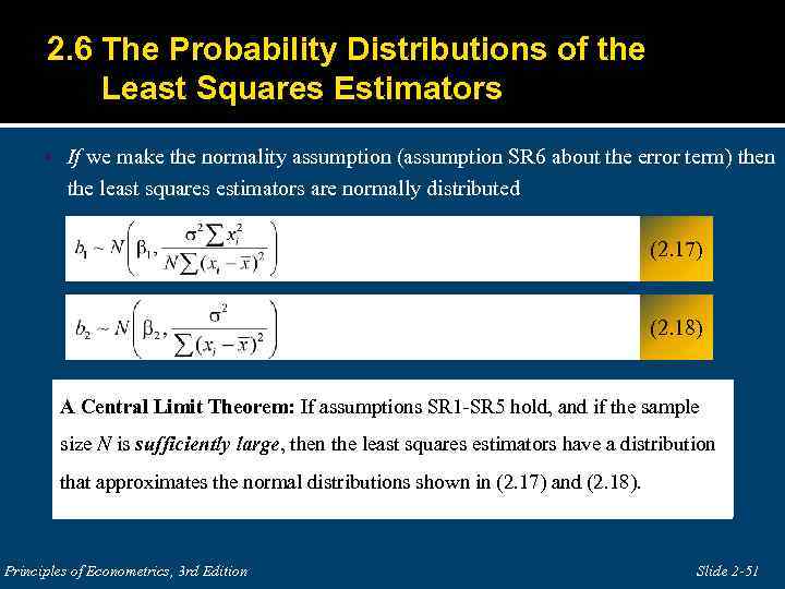2. 6 The Probability Distributions of the Least Squares Estimators If we make the normality assumption (assumption SR 6 about the error term) then the least squares estimators are normally distributed (2. 17) (2. 18) A Central Limit Theorem: If assumptions SR 1 -SR 5 hold, and if the sample size N is sufficiently large, then the least squares estimators have a distribution that approximates the normal distributions shown in (2. 17) and (2. 18). Principles of Econometrics, 3 rd Edition Slide 2 -51

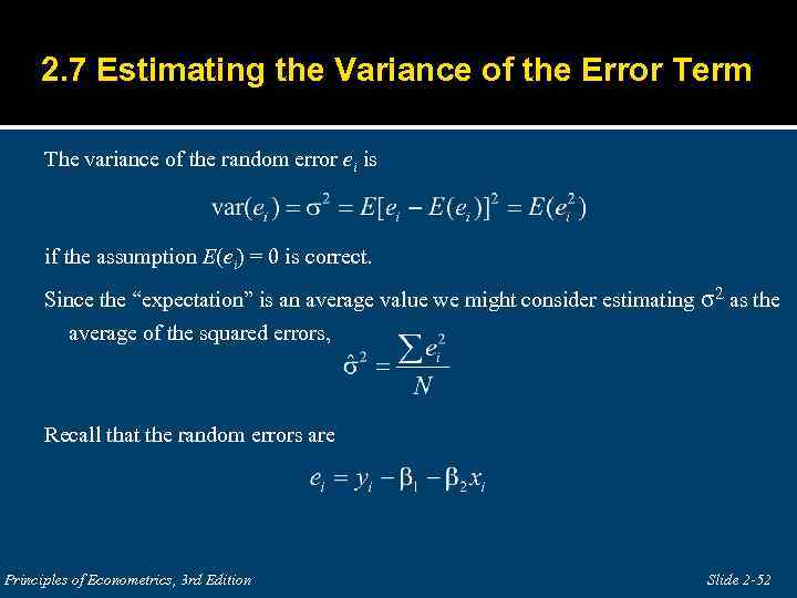2. 7 Estimating the Variance of the Error Term The variance of the random error ei is if the assumption E(ei) = 0 is correct. Since the “expectation” is an average value we might consider estimating σ2 as the average of the squared errors, Recall that the random errors are Principles of Econometrics, 3 rd Edition Slide 2 -52

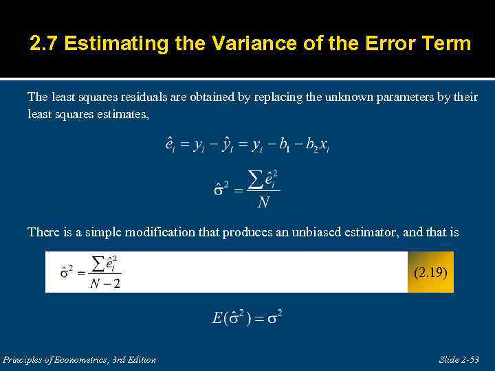2. 7 Estimating the Variance of the Error Term The least squares residuals are obtained by replacing the unknown parameters by their least squares estimates, There is a simple modification that produces an unbiased estimator, and that is (2. 19) Principles of Econometrics, 3 rd Edition Slide 2 -53

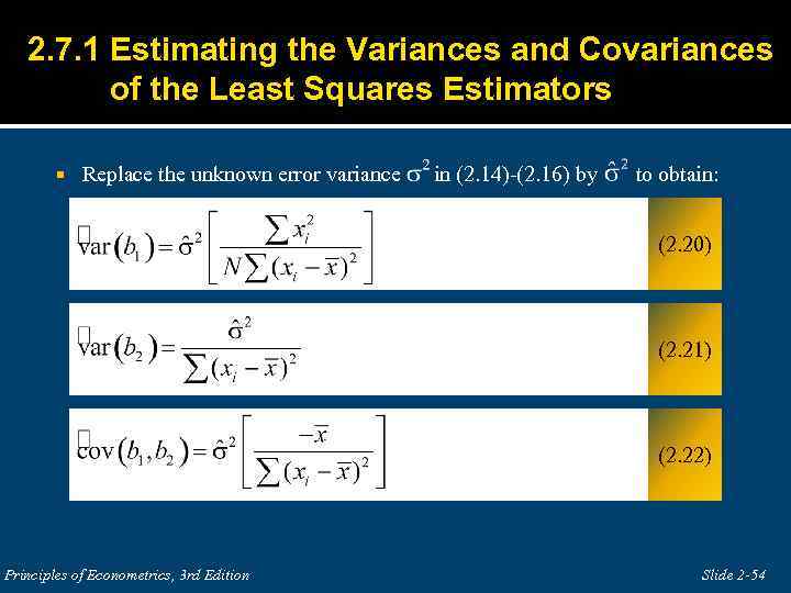2. 7. 1 Estimating the Variances and Covariances of the Least Squares Estimators Replace the unknown error variance in (2. 14)-(2. 16) by to obtain: (2. 20) (2. 21) (2. 22) Principles of Econometrics, 3 rd Edition Slide 2 -54

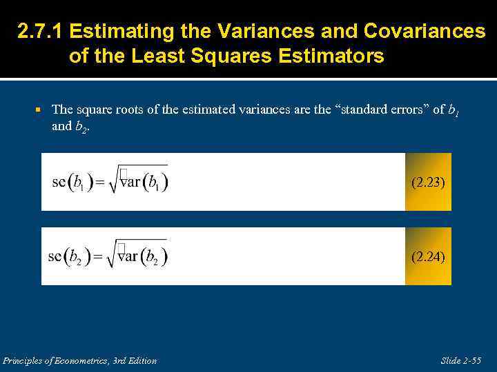2. 7. 1 Estimating the Variances and Covariances of the Least Squares Estimators The square roots of the estimated variances are the “standard errors” of b 1 and b 2. (2. 23) (2. 24) Principles of Econometrics, 3 rd Edition Slide 2 -55

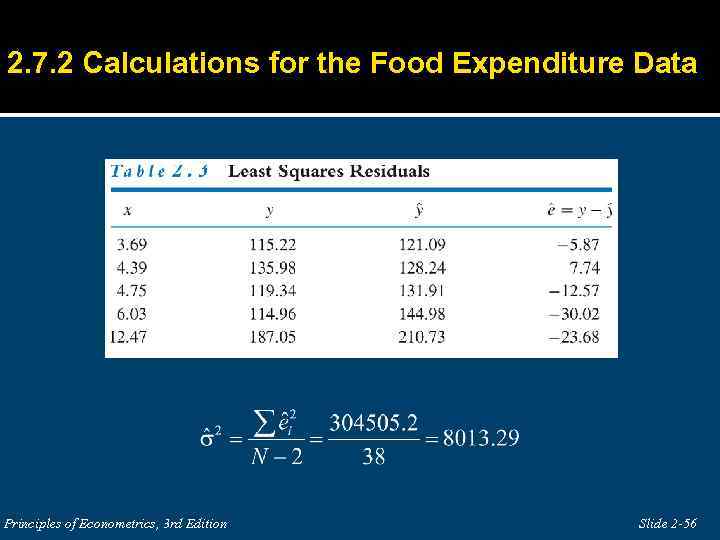2. 7. 2 Calculations for the Food Expenditure Data Principles of Econometrics, 3 rd Edition Slide 2 -56

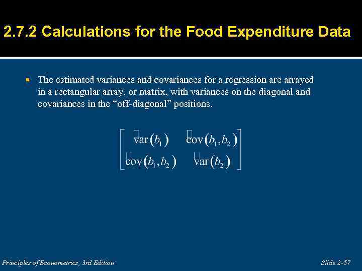2. 7. 2 Calculations for the Food Expenditure Data The estimated variances and covariances for a regression are arrayed in a rectangular array, or matrix, with variances on the diagonal and covariances in the “off-diagonal” positions. Principles of Econometrics, 3 rd Edition Slide 2 -57

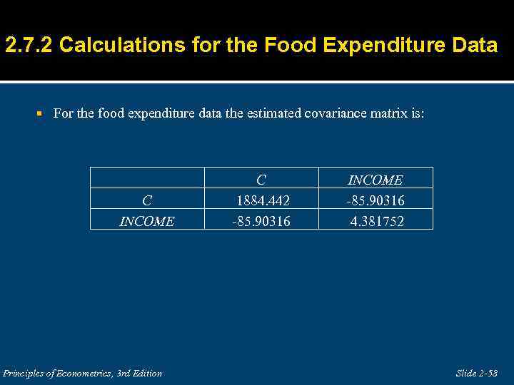2. 7. 2 Calculations for the Food Expenditure Data For the food expenditure data the estimated covariance matrix is: C INCOME Principles of Econometrics, 3 rd Edition C 1884. 442 -85. 90316 INCOME -85. 90316 4. 381752 Slide 2 -58

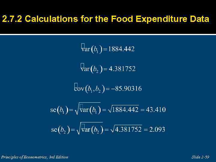2. 7. 2 Calculations for the Food Expenditure Data Principles of Econometrics, 3 rd Edition Slide 2 -59

Keywords assumptions asymptotic B. L. U. E. biased estimator degrees of freedom dependent variable deviation from the mean form econometric model economic model elasticity Gauss-Markov Theorem heteroskedastic Principles of Econometrics, 3 rd Edition homoskedastic independent variable least squares estimates least squares estimators least squares principle least squares residuals linear estimator prediction random error term regression model regression parameters repeated sampling precision sampling properties scatter diagram simple linear regression function specification error unbiased estimator Slide 2 -60

Chapter 2 Appendices Appendix 2 A Derivation of the least squares estimates Appendix 2 B Deviation from the mean form of b 2 Appendix 2 C b 2 is a linear estimator Appendix 2 D Derivation of Theoretical Expression for b 2 Appendix 2 E Deriving the variance of b 2 Appendix 2 F Proof of the Gauss-Markov Theorem Principles of Econometrics, 3 rd Edition Slide 2 -61

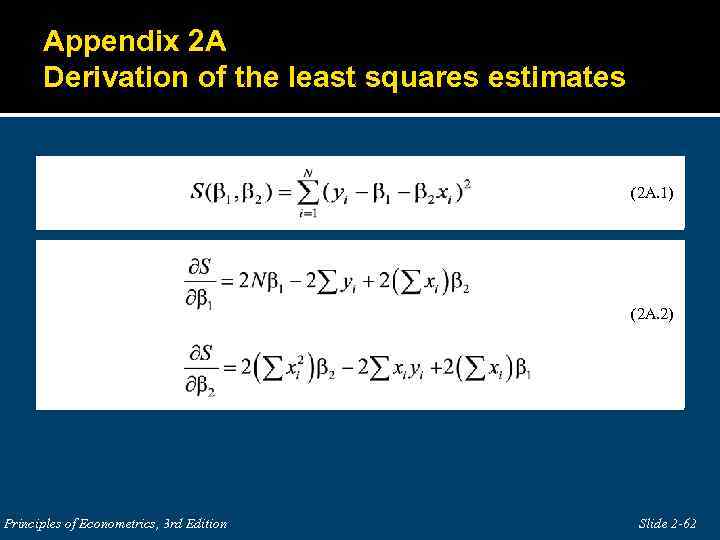Appendix 2 A Derivation of the least squares estimates (2 A. 1) (2 A. 2) Principles of Econometrics, 3 rd Edition Slide 2 -62

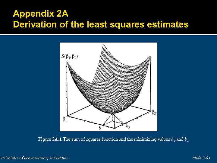Appendix 2 A Derivation of the least squares estimates Figure 2 A. 1 The sum of squares function and the minimizing values b 1 and b 2 Principles of Econometrics, 3 rd Edition Slide 2 -63

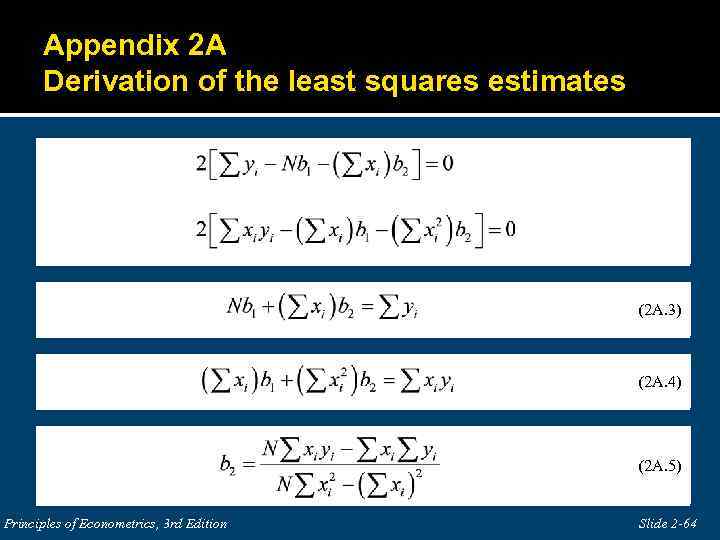Appendix 2 A Derivation of the least squares estimates (2 A. 3) (2 A. 4) (2 A. 5) Principles of Econometrics, 3 rd Edition Slide 2 -64

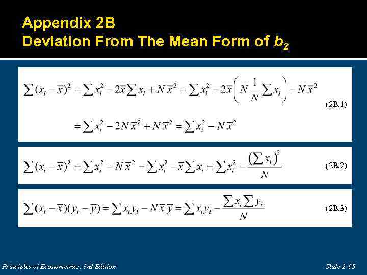Appendix 2 B Deviation From The Mean Form of b 2 (2 B. 1) (2 B. 2) (2 B. 3) Principles of Econometrics, 3 rd Edition Slide 2 -65

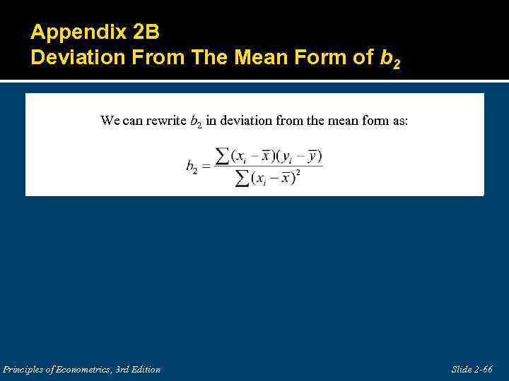Appendix 2 B Deviation From The Mean Form of b 2 We can rewrite b 2 in deviation from the mean form as: Principles of Econometrics, 3 rd Edition Slide 2 -66

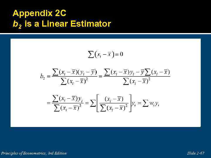Appendix 2 C b 2 is a Linear Estimator Principles of Econometrics, 3 rd Edition Slide 2 -67

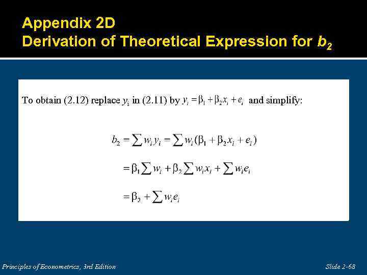Appendix 2 D Derivation of Theoretical Expression for b 2 To obtain (2. 12) replace yi in (2. 11) by and simplify: Principles of Econometrics, 3 rd Edition Slide 2 -68

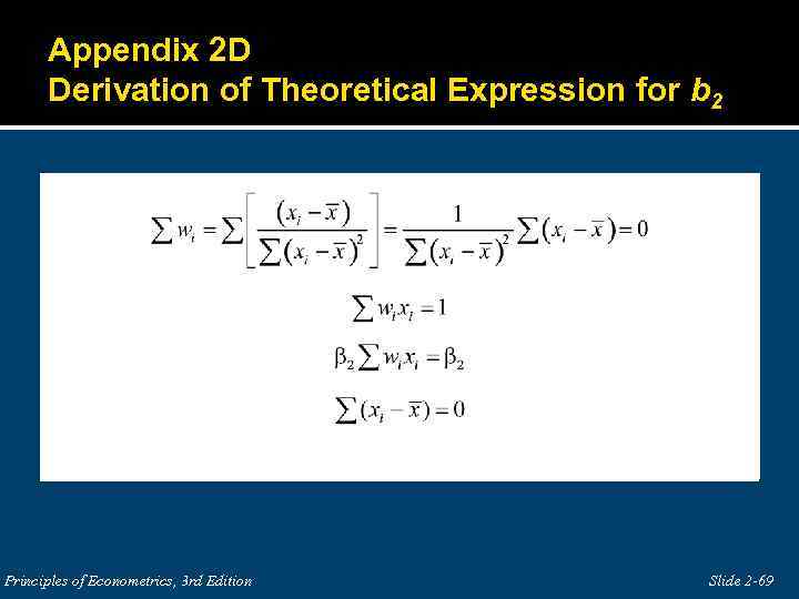Appendix 2 D Derivation of Theoretical Expression for b 2 Principles of Econometrics, 3 rd Edition Slide 2 -69

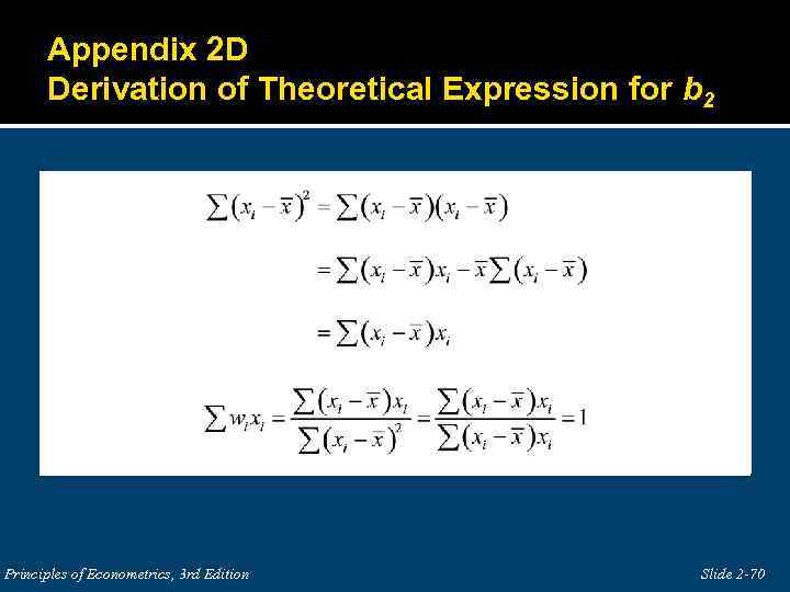Appendix 2 D Derivation of Theoretical Expression for b 2 Principles of Econometrics, 3 rd Edition Slide 2 -70

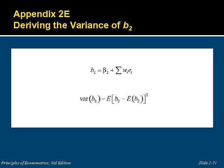Appendix 2 E Deriving the Variance of b 2 Principles of Econometrics, 3 rd Edition Slide 2 -71

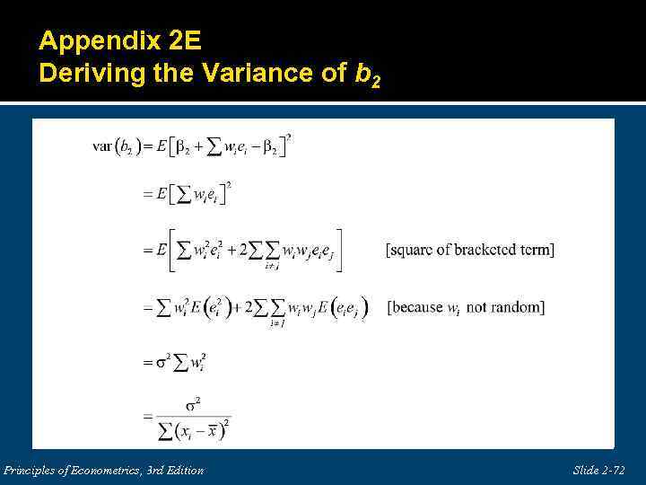Appendix 2 E Deriving the Variance of b 2 Principles of Econometrics, 3 rd Edition Slide 2 -72

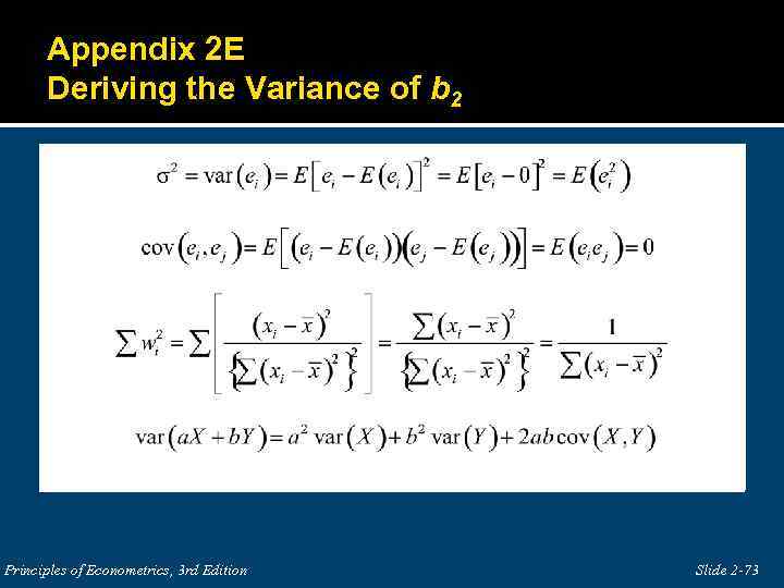Appendix 2 E Deriving the Variance of b 2 Principles of Econometrics, 3 rd Edition Slide 2 -73

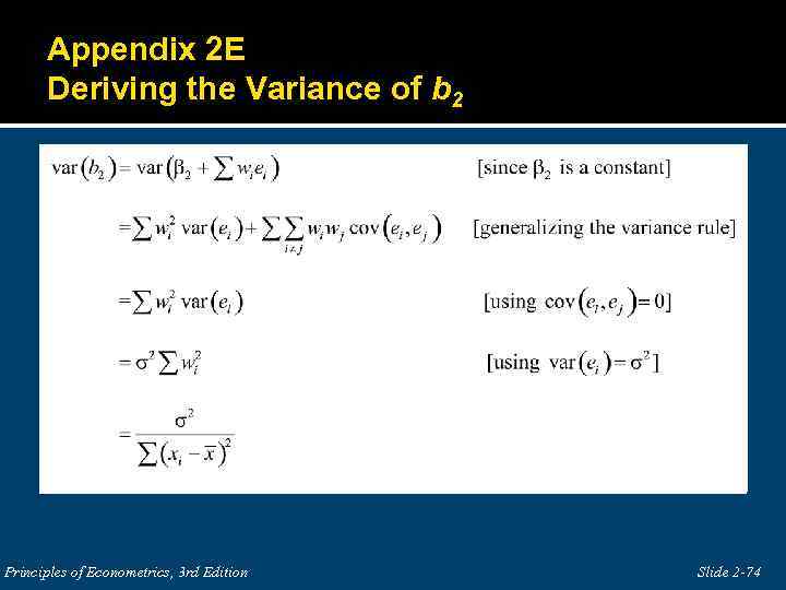Appendix 2 E Deriving the Variance of b 2 Principles of Econometrics, 3 rd Edition Slide 2 -74

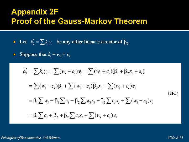Appendix 2 F Proof of the Gauss-Markov Theorem Let be any other linear estimator of β 2. Suppose that ki = wi + ci. (2 F. 1) Principles of Econometrics, 3 rd Edition Slide 2 -75

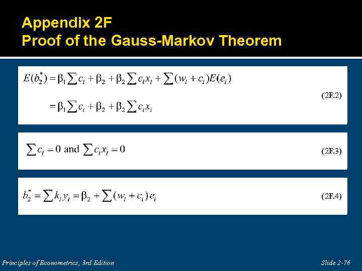Appendix 2 F Proof of the Gauss-Markov Theorem (2 F. 2) (2 F. 3) (2 F. 4) Principles of Econometrics, 3 rd Edition Slide 2 -76

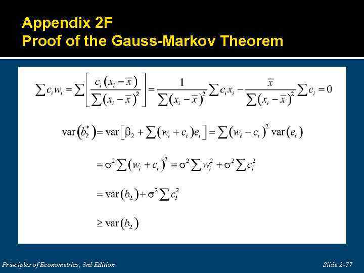Appendix 2 F Proof of the Gauss-Markov Theorem Principles of Econometrics, 3 rd Edition Slide 2 -77