THE MATHEMATICS OF CAUSAL INFERENCE IN STATISTICS Judea

THE MATHEMATICS OF CAUSAL INFERENCE IN STATISTICS Judea Pearl Department of Computer Science UCLA

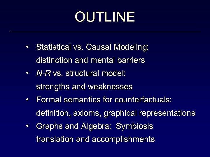OUTLINE • Statistical vs. Causal Modeling: distinction and mental barriers • N-R vs. structural model: strengths and weaknesses • Formal semantics for counterfactuals: definition, axioms, graphical representations • Graphs and Algebra: Symbiosis translation and accomplishments

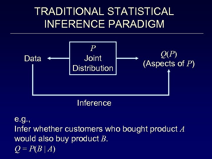TRADITIONAL STATISTICAL INFERENCE PARADIGM Data P Joint Distribution Q(P) (Aspects of P) Inference e. g. , Infer whether customers who bought product A would also buy product B. Q = P(B | A)

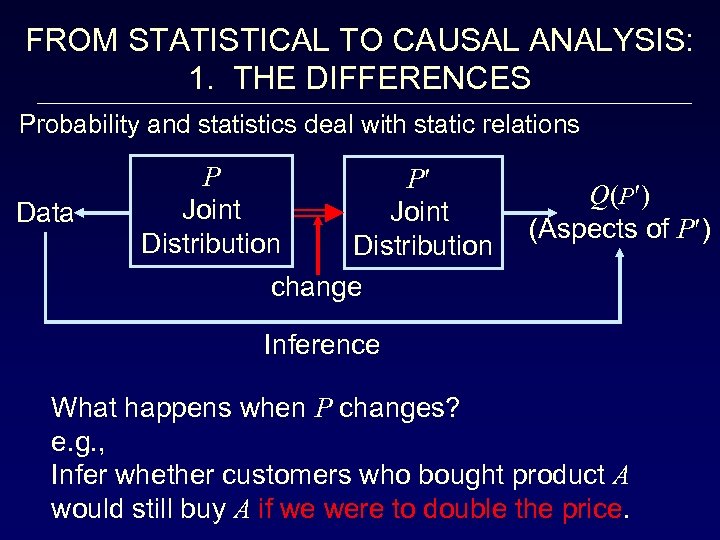FROM STATISTICAL TO CAUSAL ANALYSIS: 1. THE DIFFERENCES Probability and statistics deal with static relations Data P Joint Distribution change Q(P ) (Aspects of P ) Inference What happens when P changes? e. g. , Infer whether customers who bought product A would still buy A if we were to double the price.

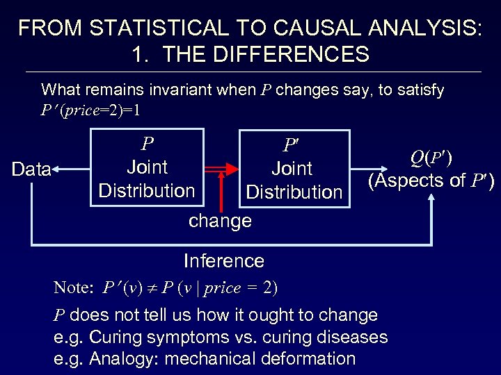FROM STATISTICAL TO CAUSAL ANALYSIS: 1. THE DIFFERENCES What remains invariant when P changes say, to satisfy P (price=2)=1 Data P Joint Distribution change Q(P ) (Aspects of P ) Inference Note: P (v) P (v | price = 2) P does not tell us how it ought to change e. g. Curing symptoms vs. curing diseases e. g. Analogy: mechanical deformation

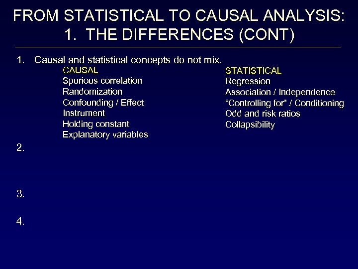FROM STATISTICAL TO CAUSAL ANALYSIS: 1. THE DIFFERENCES (CONT) 1. Causal and statistical concepts do not mix. CAUSAL Spurious correlation Randomization Confounding / Effect Instrument Holding constant Explanatory variables 2. 3. 4. STATISTICAL Regression Association / Independence “Controlling for” / Conditioning Odd and risk ratios Collapsibility

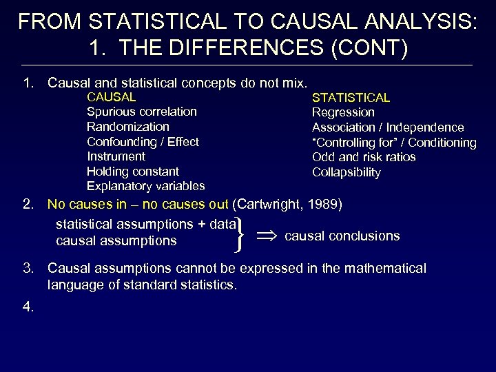FROM STATISTICAL TO CAUSAL ANALYSIS: 1. THE DIFFERENCES (CONT) 1. Causal and statistical concepts do not mix. CAUSAL Spurious correlation Randomization Confounding / Effect Instrument Holding constant Explanatory variables STATISTICAL Regression Association / Independence “Controlling for” / Conditioning Odd and risk ratios Collapsibility 2. No causes in – no causes out (Cartwright, 1989) statistical assumptions + data causal conclusions causal assumptions } 3. Causal assumptions cannot be expressed in the mathematical language of standard statistics. 4.

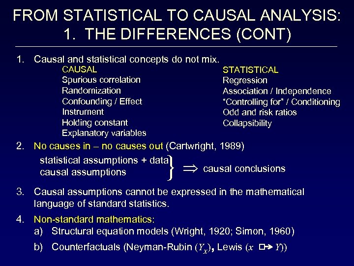FROM STATISTICAL TO CAUSAL ANALYSIS: 1. THE DIFFERENCES (CONT) 1. Causal and statistical concepts do not mix. CAUSAL Spurious correlation Randomization Confounding / Effect Instrument Holding constant Explanatory variables STATISTICAL Regression Association / Independence “Controlling for” / Conditioning Odd and risk ratios Collapsibility 2. No causes in – no causes out (Cartwright, 1989) statistical assumptions + data causal conclusions causal assumptions } 3. Causal assumptions cannot be expressed in the mathematical language of standard statistics. 4. Non-standard mathematics: a) Structural equation models (Wright, 1920; Simon, 1960) b) Counterfactuals (Neyman-Rubin (Yx), Lewis (x Y))

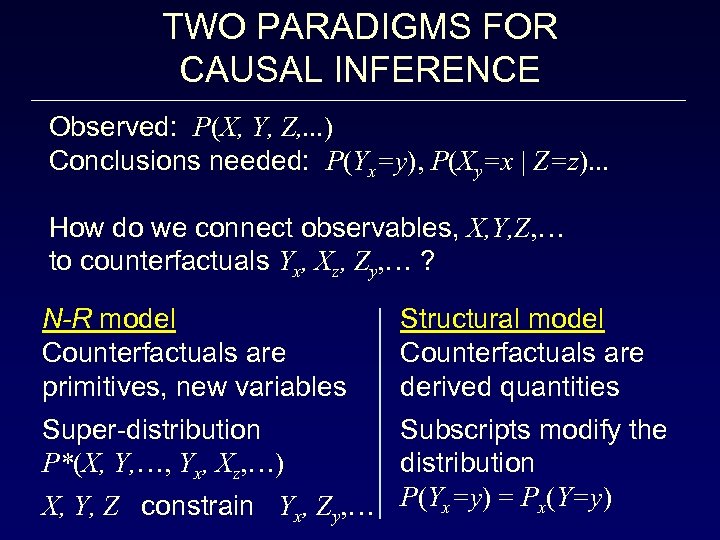TWO PARADIGMS FOR CAUSAL INFERENCE Observed: P(X, Y, Z, . . . ) Conclusions needed: P(Yx=y), P(Xy=x | Z=z). . . How do we connect observables, X, Y, Z, … to counterfactuals Yx, Xz, Zy, … ? N-R model Counterfactuals are primitives, new variables Super-distribution P*(X, Y, …, Yx, Xz, …) Structural model Counterfactuals are derived quantities Subscripts modify the distribution X, Y, Z constrain Yx, Zy, … P(Yx=y) = Px(Y=y)

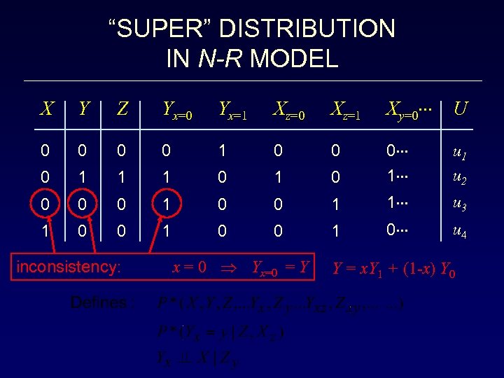“SUPER” DISTRIBUTION IN N-R MODEL X Y Z Yx=0 Yx=1 Xz=0 Xz=1 Xy=0 U 0 0 1 0 0 0 1 1 1 0 0 1 u 2 0 0 0 1 1 u 3 1 0 0 1 0 u 4 inconsistency: x = 0 Yx=0 = Y Y = x. Y 1 + (1 -x) Y 0

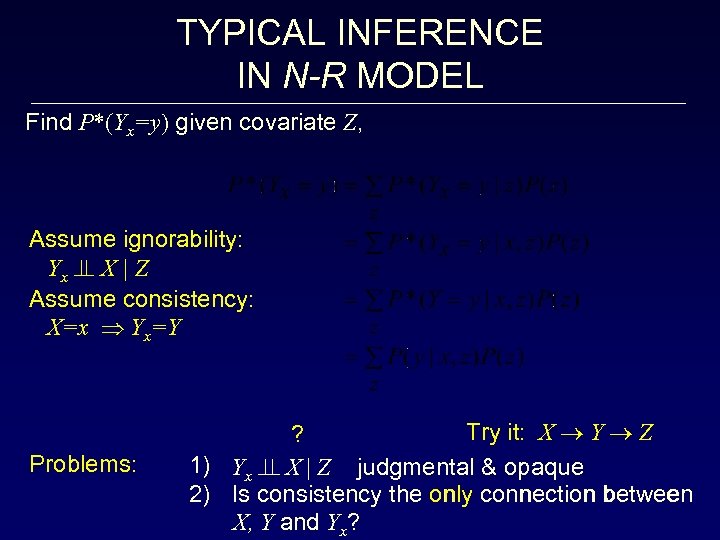TYPICAL INFERENCE IN N-R MODEL Find P*(Yx=y) given covariate Z, Assume ignorability: Yx X | Z Assume consistency: X=x Yx=Y Problems: Try it: X Y Z ? 1) Yx X | Z judgmental & opaque 2) Is consistency the only connection between X, Y and Yx?

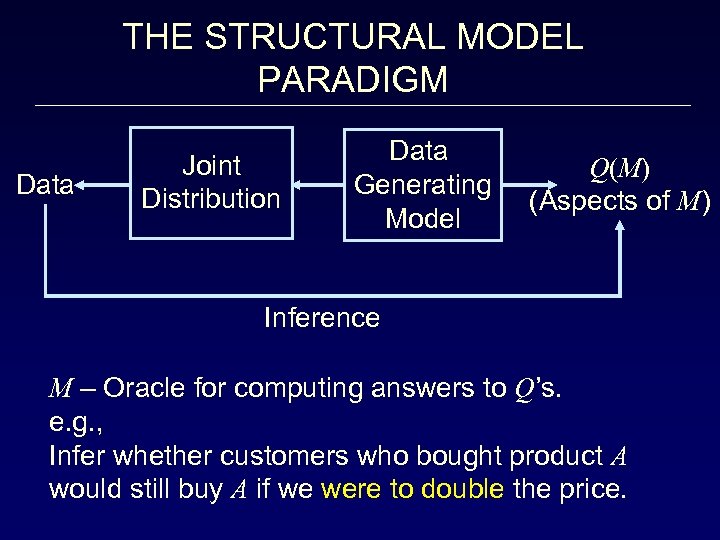THE STRUCTURAL MODEL PARADIGM Data Joint Distribution Data Generating Model Q(M) (Aspects of M) Inference M – Oracle for computing answers to Q’s. e. g. , Infer whether customers who bought product A would still buy A if we were to double the price.

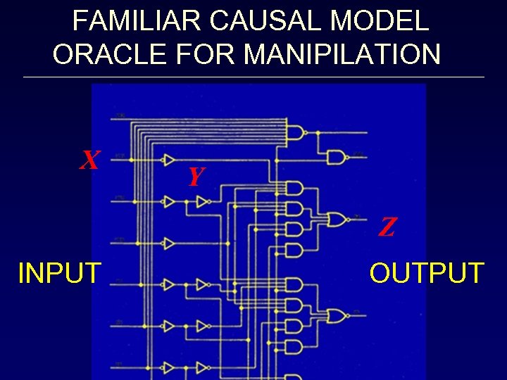FAMILIAR CAUSAL MODEL ORACLE FOR MANIPILATION X Y Z INPUT OUTPUT

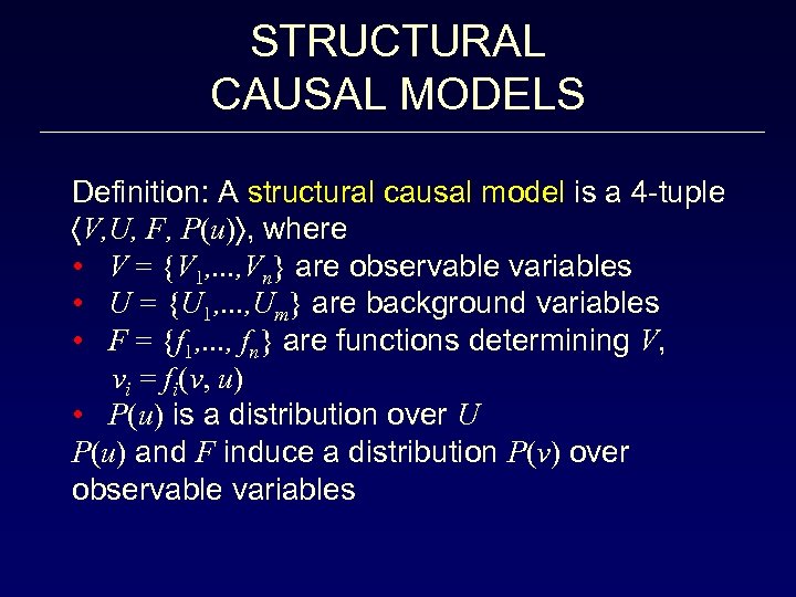STRUCTURAL CAUSAL MODELS Definition: A structural causal model is a 4 -tuple V, U, F, P(u) , where • V = {V 1, . . . , Vn} are observable variables • U = {U 1, . . . , Um} are background variables • F = {f 1, . . . , fn} are functions determining V, vi = fi(v, u) • P(u) is a distribution over U P(u) and F induce a distribution P(v) over observable variables

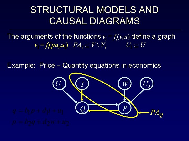STRUCTURAL MODELS AND CAUSAL DIAGRAMS The arguments of the functions vi = fi(v, u) define a graph vi = fi(pai, ui) PAi V Vi Ui U Example: Price – Quantity equations in economics U 1 I W Q P U 2 PAQ

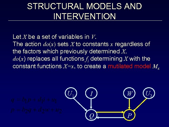STRUCTURAL MODELS AND INTERVENTION Let X be a set of variables in V. The action do(x) sets X to constants x regardless of the factors which previously determined X. do(x) replaces all functions fi determining X with the constant functions X=x, to create a mutilated model Mx U 1 I W Q P U 2

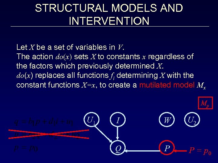STRUCTURAL MODELS AND INTERVENTION Let X be a set of variables in V. The action do(x) sets X to constants x regardless of the factors which previously determined X. do(x) replaces all functions fi determining X with the constant functions X=x, to create a mutilated model Mx Mp U 1 I W U 2 Q P P = p 0

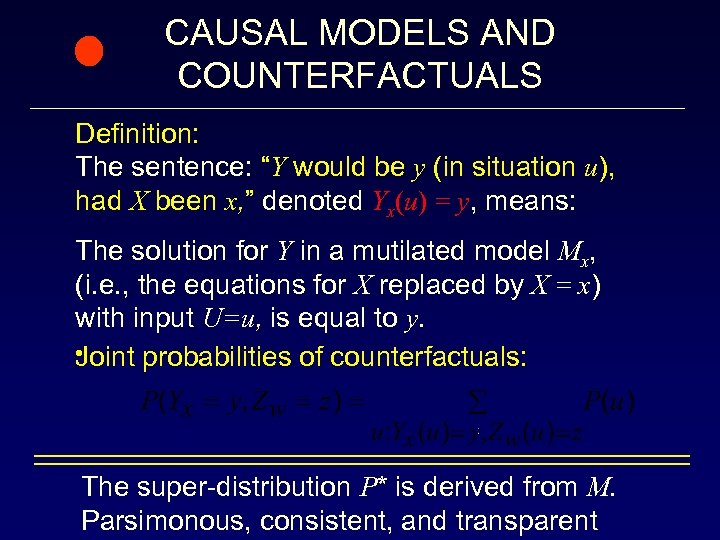CAUSAL MODELS AND COUNTERFACTUALS Definition: The sentence: “Y would be y (in situation u), had X been x, ” denoted Yx(u) = y, means: The solution for Y in a mutilated model Mx, (i. e. , the equations for X replaced by X = x) with input U=u, is equal to y. • Joint probabilities of counterfactuals: The super-distribution P* is derived from M. Parsimonous, consistent, and transparent

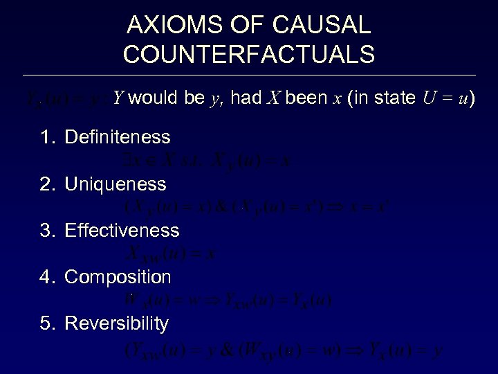AXIOMS OF CAUSAL COUNTERFACTUALS Y would be y, had X been x (in state U = u) 1. Definiteness 2. Uniqueness 3. Effectiveness 4. Composition 5. Reversibility

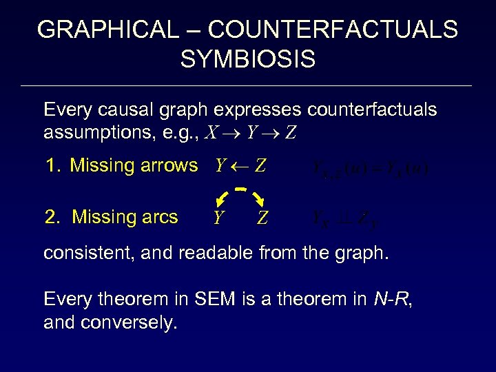GRAPHICAL – COUNTERFACTUALS SYMBIOSIS Every causal graph expresses counterfactuals assumptions, e. g. , X Y Z 1. Missing arrows Y Z 2. Missing arcs Y Z consistent, and readable from the graph. Every theorem in SEM is a theorem in N-R, and conversely.

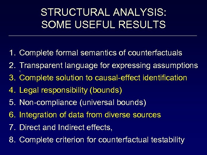STRUCTURAL ANALYSIS: SOME USEFUL RESULTS 1. Complete formal semantics of counterfactuals 2. Transparent language for expressing assumptions 1. 3. Complete solution to causal-effect identification 4. Legal responsibility (bounds) 5. Non-compliance (universal bounds) 6. Integration of data from diverse sources 7. Direct and Indirect effects, 8. Complete criterion for counterfactual testability

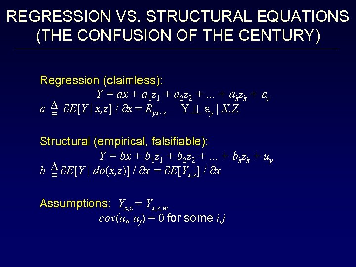REGRESSION VS. STRUCTURAL EQUATIONS (THE CONFUSION OF THE CENTURY) Regression (claimless): Y = ax + a 1 z 1 + a 2 z 2 +. . . + akzk + y a E[Y | x, z] / x = Ryx z Y y | X, Z = Structural (empirical, falsifiable): Y = bx + b 1 z 1 + b 2 z 2 +. . . + bkzk + uy b E[Y | do(x, z)] / x = E[Yx, z] / x = Assumptions: Yx, z = Yx, z, w cov(ui, uj) = 0 for some i, j

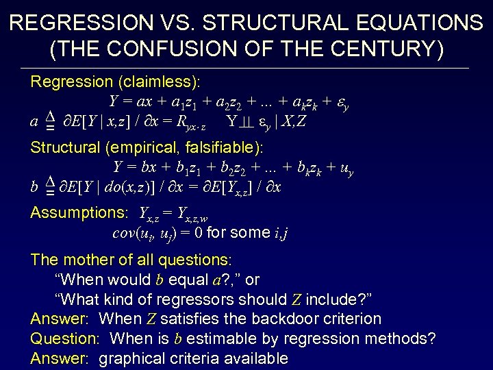REGRESSION VS. STRUCTURAL EQUATIONS (THE CONFUSION OF THE CENTURY) Regression (claimless): Y = ax + a 1 z 1 + a 2 z 2 +. . . + akzk + y a E[Y | x, z] / x = Ryx z Y y | X, Z = Structural (empirical, falsifiable): Y = bx + b 1 z 1 + b 2 z 2 +. . . + bkzk + uy b E[Y | do(x, z)] / x = E[Yx, z] / x = Assumptions: Yx, z = Yx, z, w cov(ui, uj) = 0 for some i, j The mother of all questions: “When would b equal a? , ” or “What kind of regressors should Z include? ” Answer: When Z satisfies the backdoor criterion Question: When is b estimable by regression methods? Answer: graphical criteria available

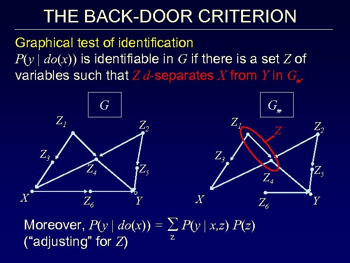THE BACK-DOOR CRITERION Graphical test of identification P(y | do(x)) is identifiable in G if there is a set Z of variables such that Z d-separates X from Y in Gx. G Z 1 Z 3 X Gx Z 1 Z 2 Z 4 Z 6 Z 3 Z 5 Y Z Z 4 X Moreover, P(y | do(x)) = å P(y | x, z) P(z) z (“adjusting” for Z) Z 6 Z 2 Z 5 Y

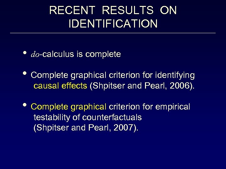RECENT RESULTS ON IDENTIFICATION • do-calculus is complete • Complete graphical criterion for identifying causal effects (Shpitser and Pearl, 2006). • Complete graphical criterion for empirical testability of counterfactuals (Shpitser and Pearl, 2007).

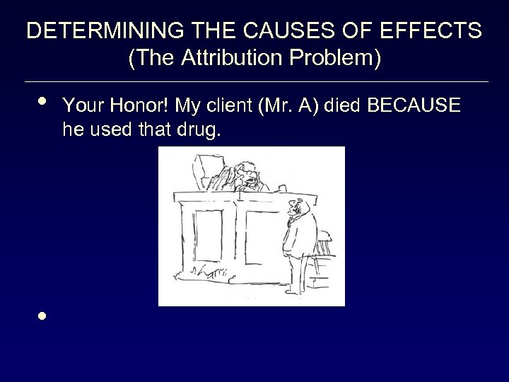DETERMINING THE CAUSES OF EFFECTS (The Attribution Problem) • • Your Honor! My client (Mr. A) died BECAUSE he used that drug.

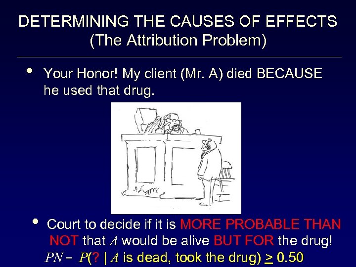DETERMINING THE CAUSES OF EFFECTS (The Attribution Problem) • • Your Honor! My client (Mr. A) died BECAUSE he used that drug. Court to decide if it is MORE PROBABLE THAN NOT that A would be alive BUT FOR the drug! PN = P(? | A is dead, took the drug) > 0. 50

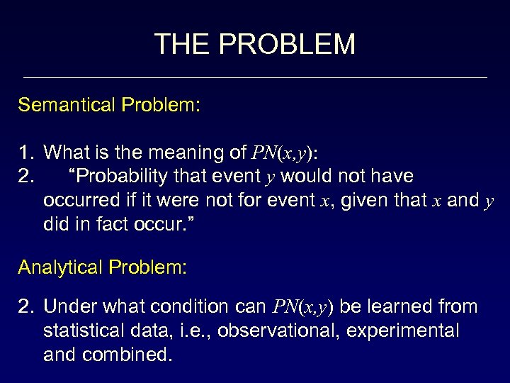
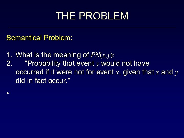THE PROBLEM Semantical Problem: 1. What is the meaning of PN(x, y): 2. “Probability that event y would not have occurred if it were not for event x, given that x and y did in fact occur. ” •

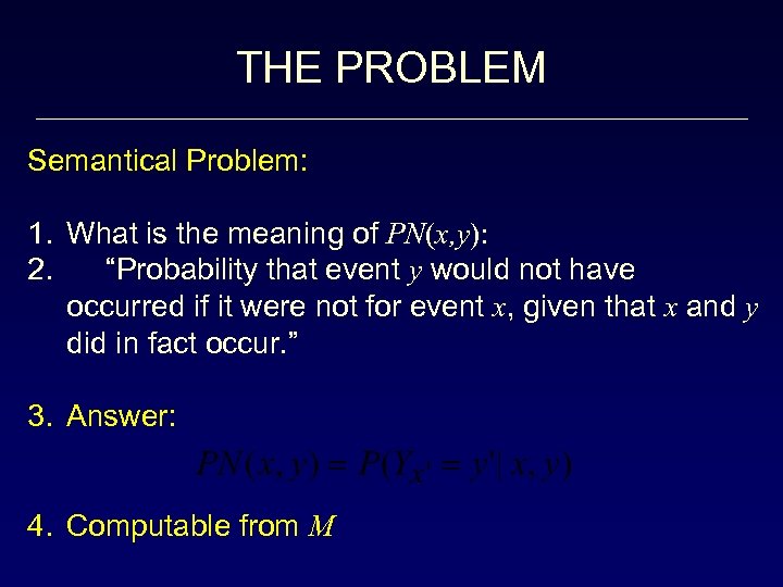THE PROBLEM Semantical Problem: 1. What is the meaning of PN(x, y): 2. “Probability that event y would not have occurred if it were not for event x, given that x and y did in fact occur. ” 3. Answer: 4. Computable from M

THE PROBLEM Semantical Problem: 1. What is the meaning of PN(x, y): 2. “Probability that event y would not have occurred if it were not for event x, given that x and y did in fact occur. ” Analytical Problem: 2. Under what condition can PN(x, y) be learned from statistical data, i. e. , observational, experimental and combined.

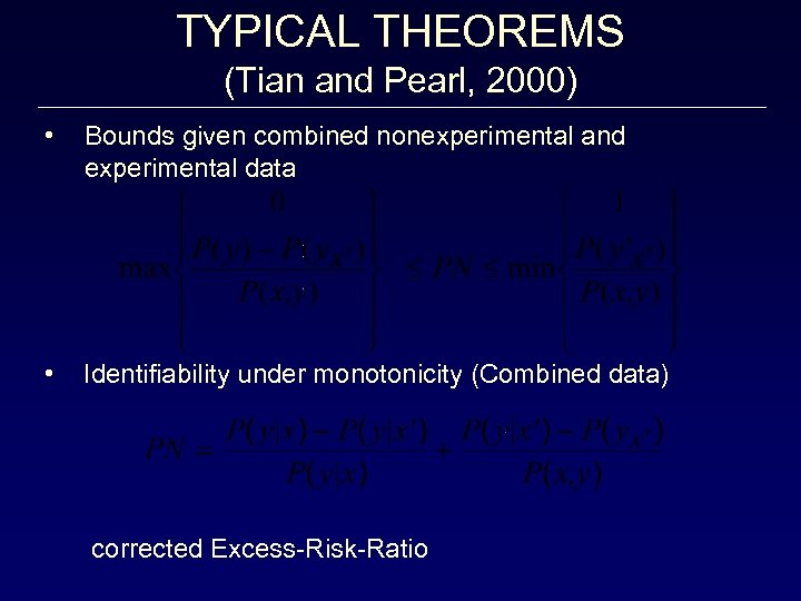TYPICAL THEOREMS (Tian and Pearl, 2000) • Bounds given combined nonexperimental and experimental data • Identifiability under monotonicity (Combined data) corrected Excess-Risk-Ratio

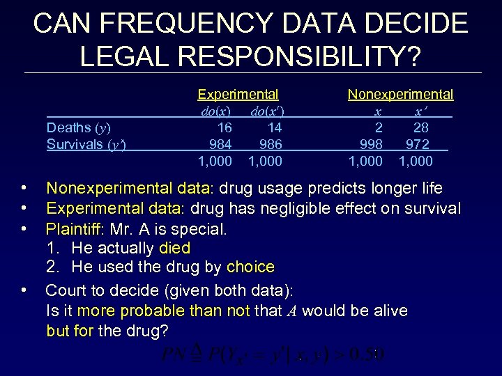CAN FREQUENCY DATA DECIDE LEGAL RESPONSIBILITY? Deaths (y) Survivals (y ) • • Experimental do(x) do(x ) 16 14 986 1, 000 Nonexperimental x x 2 28 998 972 1, 000 Nonexperimental data: drug usage predicts longer life Experimental data: drug has negligible effect on survival Plaintiff: Mr. A is special. 1. He actually died 2. He used the drug by choice Court to decide (given both data): Is it more probable than not that A would be alive but for the drug?

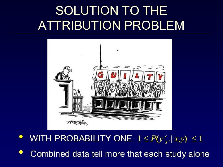SOLUTION TO THE ATTRIBUTION PROBLEM • • WITH PROBABILITY ONE 1 P(y x | x, y) 1 Combined data tell more that each study alone

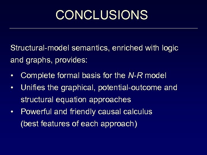CONCLUSIONS Structural-model semantics, enriched with logic and graphs, provides: • Complete formal basis for the N-R model • Unifies the graphical, potential-outcome and structural equation approaches • Powerful and friendly causal calculus (best features of each approach)