The Macroeconomics of housing markets Session 1 A

“The Macroeconomics of housing markets” Session 1 A: Housing and the business cycle - Domestic features HOUSING AND THE MACROECONOMY: THE ITALIAN CASE Guido Bulligan* Paris, 3 -4 December 2009 * Bank of Italy, Department of Economic Outlook and Monetary Policy Studies

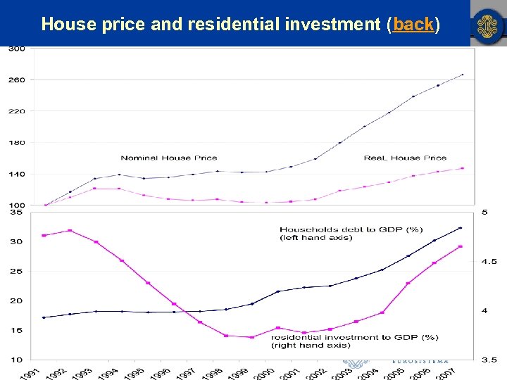
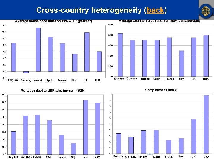
Motivations Rising housing prices, indebtedness and imbalances (graphs) • Real house prices in Italy have increased by 40% since last cyclical trough • Households debt (as % of GDP) has doubled in the last 10 years Local nature of housing markets, cross-country heterogeneity (graphs) • High home-ownership rate (72%) • Low (but increasing) level of indebtedness of Italian households • Incomplete housing finance markets (products variety, transaction costs) Empirical evidence • Existing empirical evidence mainly focused on Anglo-saxon countries

Aim of the paper Searching for stylized facts of the Italian housing market • Over the cycle: growth cycle approach • In reaction to a monetary policy shock: SVAR analysis

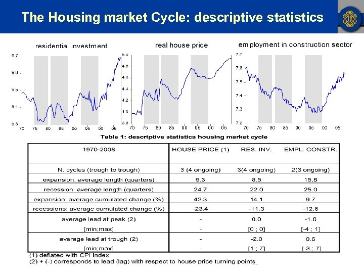The Housing market Cycle: descriptive statistics

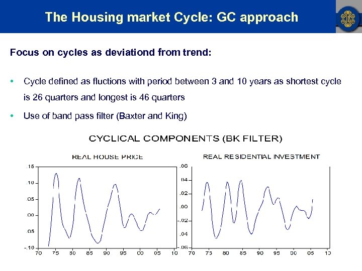The Housing market Cycle: GC approach Focus on cycles as deviationd from trend: • Cycle defined as fluctions with period between 3 and 10 years as shortest cycle is 26 quarters and longest is 46 quarters • Use of band pass filter (Baxter and King)

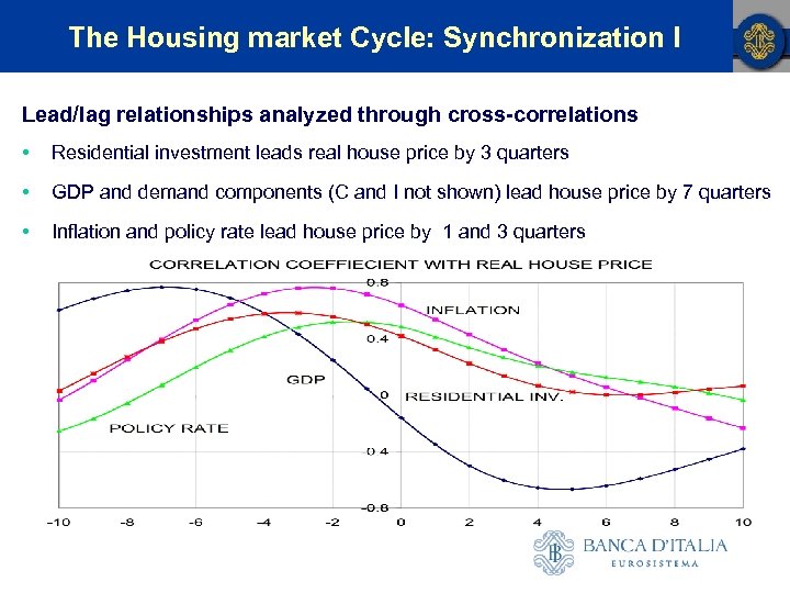The Housing market Cycle: Synchronization I Lead/lag relationships analyzed through cross-correlations • Residential investment leads real house price by 3 quarters • GDP and demand components (C and I not shown) lead house price by 7 quarters • Inflation and policy rate lead house price by 1 and 3 quarters

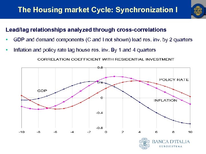The Housing market Cycle: Synchronization I Lead/lag relationships analyzed through cross-correlations • GDP and demand components (C and I not shown) lead res. inv. by 2 quarters • Inflation and policy rate lag house res. inv. By 1 and 4 quarters

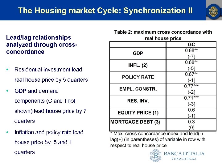The Housing market Cycle: Synchronization II Lead/lag relationships analyzed through crossconcordance • Residential investment lead real house price by 5 quarters • GDP and demand components (C and I not shown) lead house price by 7 quarters • Inflation and policy rate lead house price by 5 and 1 quarters

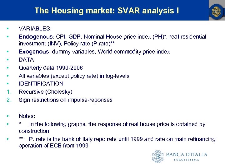The Housing market: SVAR analysis I • • 1. 2. • • • VARIABLES: Endogenous: CPI, GDP, Nominal House price index (PH)*, real residential investment (INV), Policy rate (P. rate)** Exogenous: dummy variables, World commodity price index DATA Quarterly data 1990 -2008 All variables (except policy rate) in log-levels IDENTIFICATION Recursive (Cholesky) Sign restrictions on impulse-reponses Notes: * In the following graphs, the response of real house price is obtained by construction ** P. rate is the bank of Italy repo rate until 1999 and rate on main refinancing operation of ECB from 1999

The Housing market: SVAR analysis I

The Housing market: SVAR analysis I

The Housing market: SVAR analysis II

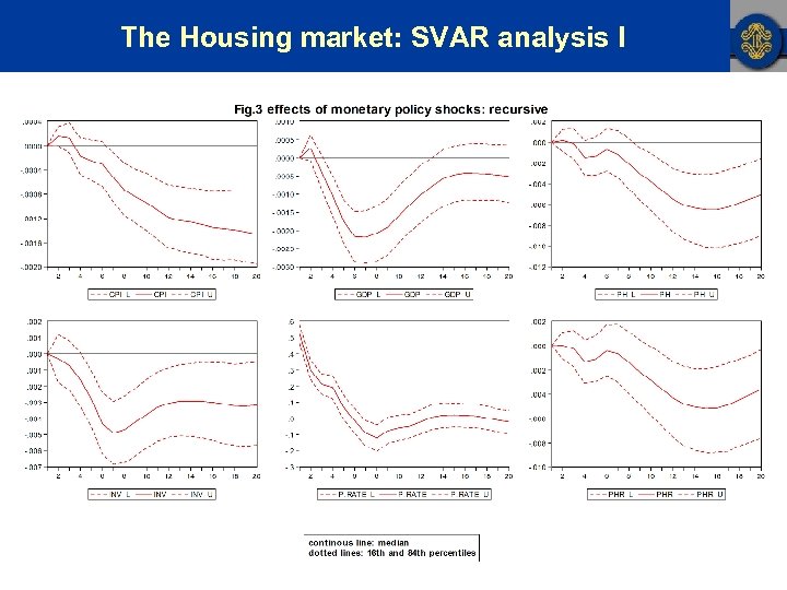
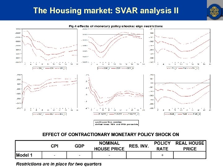
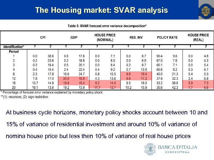The Housing market: SVAR analysis At business cycle horizons, monetary policy shocks account between 10 and 15% of variance of residential investment and around 10% of variance of nomina house price but less then 10% of variance of real house prices

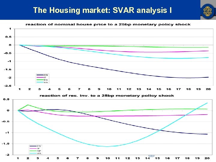
Conclusions To summarize: • Housing cycles are longer than cycles in macro variables • Housing cycles are asymmetric in terms of duration, intensity and price adjustment • GDP and components lead housing cycle • Inflation and interest rates are more coincident • Monetary policy shocks have modest but significant and long-lasting effects on housing variables (maximum impact between 0. 2% and 1% for res. investment and between 0. 1% and 0. 5% for real house price) • Monetary policy shocks explains around 10 -20 percent of variability of housing variables at the 2 -5 years horizons their role is insignificant at shorter horizons

House price and residential investment (back)

Cross-country heterogeneity (back)