The Impact of Transaction Costs and the Expected

The Impact of Transaction Costs and the Expected Length of Stay on Homeownership By Donald R. Haurin and H. Leroy Gill Journal of Urban Economics 51 Vol. 3 (2002) Presented by Shammima Jesmin

Economic Theory/Hypothesis § Economic theory/hypothesis: An increase in the expected length of stay in a dwelling increases the probability of a household choosing to own a house rather than rent. § Reason: Substantial transaction costs associated with homeownership and increased expected time in the home reduces the annualized transaction costs. (that is the transaction costs of owning are spread over a longer period). § Explanation : One part of the relationship is that the length of stay directly affects the relative cost of homeownership, which then affect tenure choice. The reciprocal relationship is that once the choice of owning or renting is made, owners recognize their greater transaction costs of relocating, causing their lengths of stay to be longer.

Authors’ Observations § Increases in aggregate rate of homeownership. § Some prior empirical works: Transaction costs used to determine tenure choice decision and Housing Mkt related Issues such as housing mkt effeiciency(Linneman: 1986), residensial mobility ( Venti and Wise 1984, Weinberg 1981), intertemporal housing adjustment model ( Harmon and potepan), housing demand mobility with transaction costs (Goodman 1995). § In most cases, transaction costs and household’s planned duration of stay in a dwelling were basically omitted from prior studies because of measurement error problem or addressed the problems in a complicated simultaneous approach. § Authors substantially overcome the problems using the new data set ( # of observations : 2621) from the 1992 Survey of the Married Military Officers and Enlisted Personnel, where the length of stay at an assigned base is known with a high degree of certainty at the time of assignment, but the choice of owning or renting is made by the military member.

What is Transaction costs? § Most easily measurable in the real estate broker’s fee - 5 -7% of the sale price of the house in U. S. A. § Implicit cost- Maintain the house in showroom condition during the time when it is on the market, searching period, transfer taxes and legal fees. § Risk bearing cost- related to maladjustment for the time of searching a new house and selling the old one. § Evidence: Goodman(1995): 5 -10% of current income, Simonson (1989): at least 6% of house value, Rosenthal (1988): 7% of house value when sold, and Linneman(1986): 12% of selling costs of homeowners,

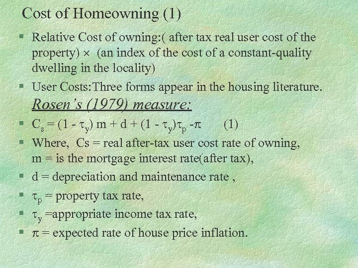Cost of Homeowning (1) § Relative Cost of owning: ( after tax real user cost of the property) (an index of the cost of a constant-quality dwelling in the locality) § User Costs: Three forms appear in the housing literature. Rosen’s (1979) measure: § Cs = (1 - y) m + d + (1 - y) p - (1) § Where, Cs = real after-tax user cost rate of owning, m = is the mortgage interest rate(after tax), § d = depreciation and maintenance rate , § p = property tax rate, § y =appropriate income tax rate, § = expected rate of house price inflation.

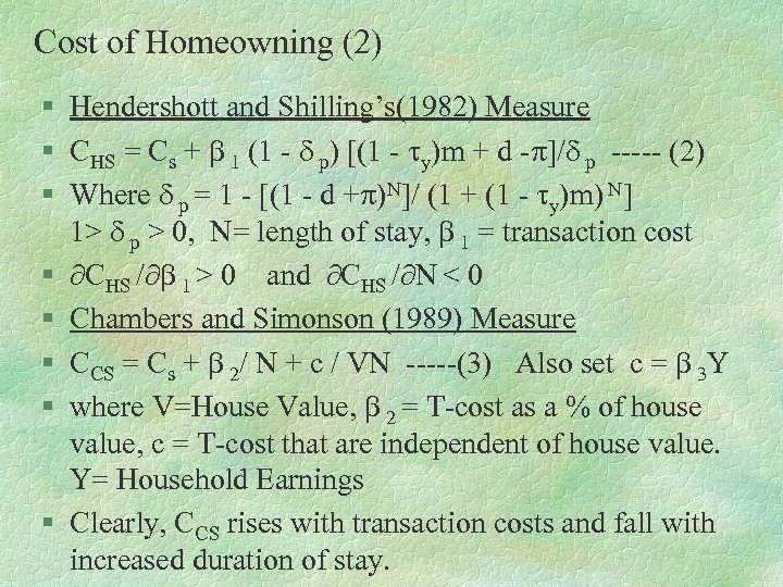Cost of Homeowning (2) § Hendershott and Shilling’s(1982) Measure § CHS = Cs + 1 (1 - p) [(1 - y)m + d - ]/ p ----- (2) § Where p = 1 - [(1 - d + )N]/ (1 + (1 - y)m) N] 1> p > 0, N= length of stay, 1 = transaction cost § CHS / 1 > 0 and CHS / N < 0 § Chambers and Simonson (1989) Measure § CCS = Cs + 2/ N + c / VN -----(3) Also set c = 3 Y § where V=House Value, 2 = T-cost as a % of house value, c = T-cost that are independent of house value. Y= Household Earnings § Clearly, CCS rises with transaction costs and fall with increased duration of stay.

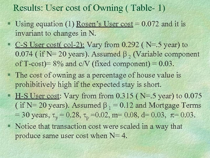Results: User cost of Owning ( Table- 1) § Using equation (1) Rosen’s User cost = 0. 072 and it is invariant to changes in N. § C-S User cost( col-2): Vary from 0. 292 ( N=. 5 year) to 0. 074 ( if N= 20 years). Assumed 2 (Variable component of T-cost)= 8% and c/V (fixed component) = 0. 03. § The cost of owning as a percentage of house value is prohibitively high if the expected stay is short. § H-S User cost: Vary from 0. 315 ( N=. 5 year) to 0. 075 ( if N= 20 years). Assumed 1 = 0. 12 and Mortgage Terms = 30 years, y = 0. 28, p =0. 02, m= 0. 08, d= 0. 03, = 0. 03. § Notice that transaction cost were scaled in a way that produce same user cost when N= 4.

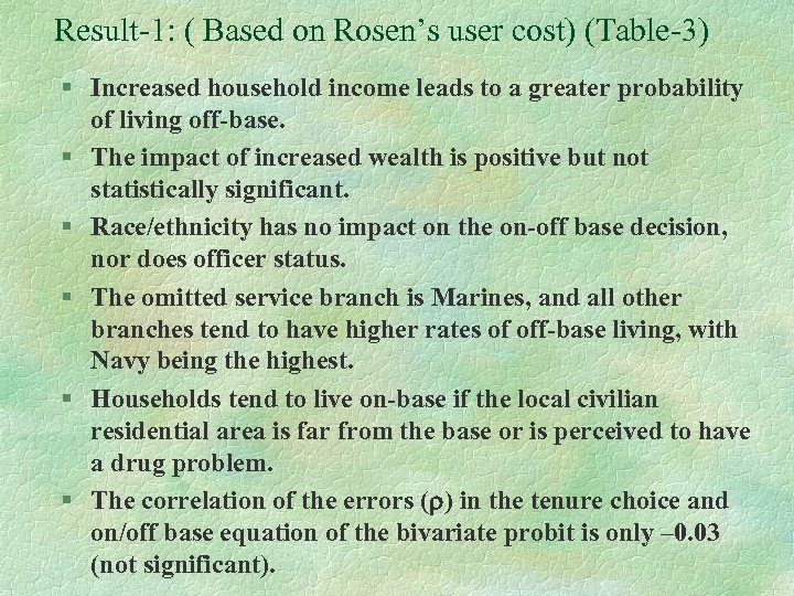Result-1: ( Based on Rosen’s user cost) (Table-3) § Increased household income leads to a greater probability of living off-base. § The impact of increased wealth is positive but not statistically significant. § Race/ethnicity has no impact on the on-off base decision, nor does officer status. § The omitted service branch is Marines, and all other branches tend to have higher rates of off-base living, with Navy being the highest. § Households tend to live on-base if the local civilian residential area is far from the base or is perceived to have a drug problem. § The correlation of the errors ( ) in the tenure choice and on/off base equation of the bivariate probit is only – 0. 03 (not significant).

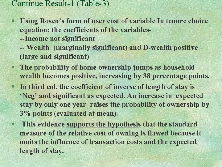Continue Result-1 (Table-3) § Using Rosen’s form of user cost of variable In tenure choice equation: the coefficients of the variables--Income not significant -- Wealth (marginally significant) and D-wealth positive (large and significant) § The probability of home ownership jumps as household wealth becomes positive, increasing by 38 percentage points. § In third col. the coefficient of inverse of length of stay is ‘Neg’ and significant as expected. An increase in expected stay by only one year raises the probability of ownership by 3% points (evaluated at mean). § This evidence supports the hypothesis that the standard measure of the relative cost of owning is flawed because it omits the influence of transaction costs and the expected length of stay.

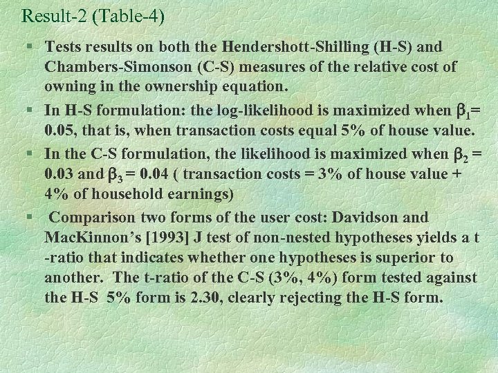Result-2 (Table-4) § Tests results on both the Hendershott-Shilling (H-S) and Chambers-Simonson (C-S) measures of the relative cost of owning in the ownership equation. § In H-S formulation: the log-likelihood is maximized when 1= 0. 05, that is, when transaction costs equal 5% of house value. § In the C-S formulation, the likelihood is maximized when 2 = 0. 03 and 3 = 0. 04 ( transaction costs = 3% of house value + 4% of household earnings) § Comparison two forms of the user cost: Davidson and Mac. Kinnon’s [1993] J test of non-nested hypotheses yields a t -ratio that indicates whether one hypotheses is superior to another. The t-ratio of the C-S (3%, 4%) form tested against the H-S 5% form is 2. 30, clearly rejecting the H-S form.

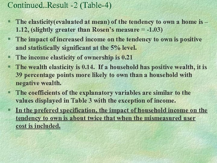Continued. . Result -2 (Table-4) § The elasticity(evaluated at mean) of the tendency to own a home is – 1. 12, (slightly greater than Rosen’s measure = -1. 03) § The impact of increased income on the tendency to own is positive and statistically significant at the 5% level. § The income elasticity of ownership is 0. 21 § The wealth elasticity is 0. 14. If a household has positive wealth, it is 39 percentage points more likely to own than a household with negative wealth. § The coefficients of the explanatory variables are similar to the values displayed in Table 3 with the exception of income. § In the prefered specification, the impact of household income on the tendency to own is about twice that when the mismeasured user cost is included.

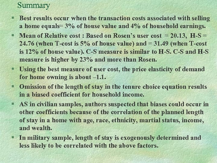Summary § Best results occur when the transaction costs associated with selling a home equals= 3% of house value and 4% of household earnings. § Mean of Relative cost : Based on Rosen’s user cost = 20. 13, H-S = 24. 76 (when T-cost is 5% of house value) and = 31. 49 (when T-cost is 12% of house value). C-S measure is similar to H-S. C-S and H-S measure is higher by 23% and more than Rosen. § Using the best measure of user cost, the price elasticity of demand for home owning is about – 1. 1. § Omission of the length of stay in the tenure choice equation results in a biased coefficient for household income. § AS in civilian samples, authors suspected that biases could occur in other coefficients because of the correlation of the planned length of stay in a home with age, race, ethnicity, martial status, income, and wealth. § In military sample, length of stay is exogenously determined and less likely to be correlated with the above factors.

Recommendations § Further researches can be done: § --to determine the appropriate size of T-costs. § -- the concept of length of stay is needed to be addressed in civilian context rather than restricted data set (because I think overall civilian plan is not so disciplined and controlled by the authority) § --Comparable study can be carried out based on planned length of stay Vs. Value of length of stay is simultaneously determined with tenure choice.