The Heckscher-Ohlin Model J Peter Neary Oxford University

The Heckscher-Ohlin Model J. Peter Neary Oxford University and CEPR

Preview: Simple General Equilibrium Models The Heckscher-Ohlin Model: • Factor-price equalisation • The Stolper-Samuelson Theorem • The Rybczynski Theorem • The Heckscher-Ohlin Theorem The Specific-Factors Model: • Comparative statics • Short-run to long-run interpretation

The Heckscher-Ohlin Model [A special case of the general competitive model] Assumptions: • • • Perfect competition, constant returns to scale 2 countries: Home and Foreign (*) 2 factors: Capital K and Labour L 2 sectors: y 1 and y 2 [Sometimes, to fix ideas: Manufacturing M and Food F] Complete intersectoral factor mobility Key Concepts: 1. Factor Abundance (of countries): • Home more labour-abundant: k < k*. 2. Factor Intensity (of industries/sectors): • Facing the same factor prices, sector 1 [M] is more capital-intensive: K 1/L 1 > K 2/L 2 or k 1 > k 2 • Assume: No "factor-intensity reversals": One sector always more capitalintensive 3

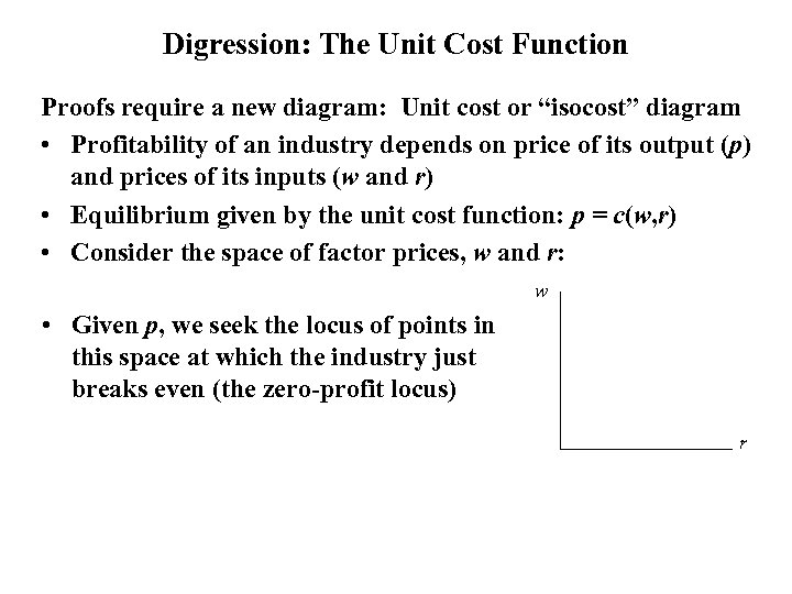Digression: The Unit Cost Function Proofs require a new diagram: Unit cost or “isocost” diagram • Profitability of an industry depends on price of its output (p) and prices of its inputs (w and r) • Equilibrium given by the unit cost function: p = c(w, r) • Consider the space of factor prices, w and r: w • Given p, we seek the locus of points in this space at which the industry just breaks even (the zero-profit locus) r

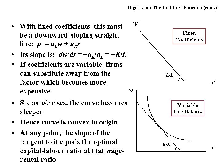Digression: The Unit Cost Function (cont. ) • With fixed coefficients, this must w be a downward-sloping straight line: p = a. Lw + a. Kr • Its slope is: dw/dr = a. K/a. L = K/L • If coefficients are variable, firms can substitute away from the factor which becomes more w expensive • So, as w/r rises, the curve becomes steeper • Hence curve is convex to origin • At any point, the slope of the tangent to it equals the optimal capital-labour ratio at that wagerental ratio Fixed Coefficients K/L r Variable Coefficients K/L r

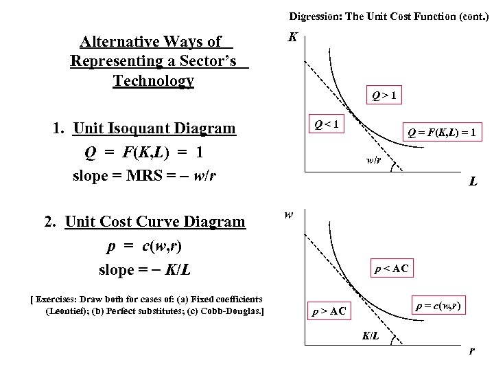Digression: The Unit Cost Function (cont. ) Alternative Ways of Representing a Sector’s Technology K Q>1 Q<1 1. Unit Isoquant Diagram Q = F(K, L) = 1 slope = MRS = w/r 2. Unit Cost Curve Diagram p = c(w, r) slope = K/L [ Exercises: Draw both for cases of: (a) Fixed coefficients (Leontief); (b) Perfect substitutes; (c) Cobb-Douglas. ] Q = F(K, L) = 1 w/r L w p < AC p = c(w, r) p > AC K/L r

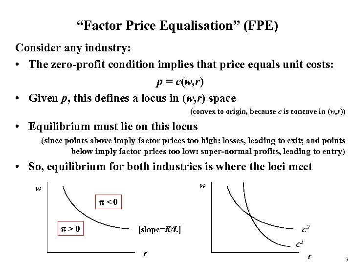“Factor Price Equalisation” (FPE) Consider any industry: • The zero-profit condition implies that price equals unit costs: p = c(w, r) • Given p, this defines a locus in (w, r) space (convex to origin, because c is concave in (w, r)) • Equilibrium must lie on this locus (since points above imply factor prices too high: losses, leading to exit; and points below imply factor prices too low: super-normal profits, leading to entry) • So, equilibrium for both industries is where the loci meet w w p<0 p>0 [slope=K/L] r c 2 c 1 r 7

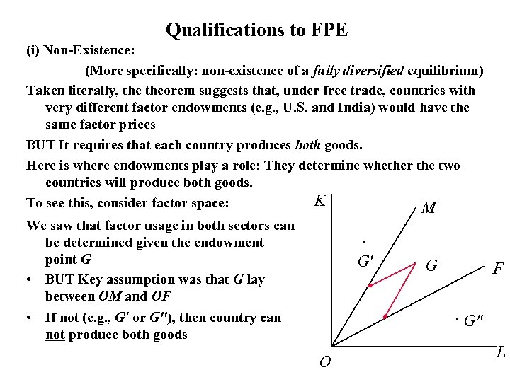Qualifications to FPE (i) Non-Existence: (More specifically: non-existence of a fully diversified equilibrium) Taken literally, theorem suggests that, under free trade, countries with very different factor endowments (e. g. , U. S. and India) would have the same factor prices BUT It requires that each country produces both goods. Here is where endowments play a role: They determine whether the two countries will produce both goods. K To see this, consider factor space: M We saw that factor usage in both sectors can be determined given the endowment point G • BUT Key assumption was that G lay between OM and OF . G' . G F . G" • If not (e. g. , G' or G"), then country can not produce both goods O L

Qualifications to FPE (cont. ) (ii) Non-Uniqueness: Factor intensity reversals are possible If: Elasticities of substitution differ enough between sectors (iii) Same number of goods and factors required: • More goods: each country may produce a different mix of goods, more suited to its own factor endowments. • More factors: Specific-factors model a simple example of a model with m > n, which rules out FPE. 9

The Stolper-Samuelson Theorem: An increase in the relative price of the capitalintensive good will increase the rental and reduce the wage, relative to the prices of both goods • Note: It refers to “real” wages and rentals • This implies that wage-earners are unambiguously worse off and capital-owners unambiguously better off

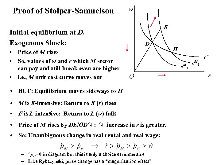Proof of Stolper-Samuelson w E Initial equilibrium at D. Exogenous Shock: • Price of M rises • So, values of w and r which M sector can pay and still break even are higher • i. e. , M unit cost curve moves out D H c. M O • BUT: Equilibrium moves sideways to H • M is K-intensive: Return to K (r) rises • F is L-intensive: Return to L (w) falls • Price of M rises by DE/OD%: % increase in r is greater. • So: Unambiguous change in real rental and real wage: – ^p. F =0 in diagram but this is only a choice of numeraire – Like Rybczynski, price change has a “magnification effect” 1 c. M 2 c. F r

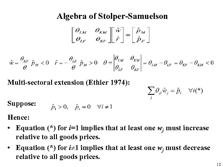Algebra of Stolper-Samuelson Multi-sectoral extension (Ethier 1974): Suppose: Hence: • Equation (*) for i=1 implies that at least one wj must increase relative to all goods prices. • Equation (*) for i¹ 1 implies that at least one wj must decrease relative to all goods prices. 12

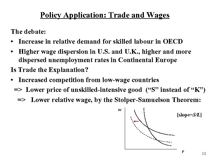Policy Application: Trade and Wages The debate: • Increase in relative demand for skilled labour in OECD • Higher wage dispersion in U. S. and U. K. , higher and more dispersed unemployment rates in Continental Europe Is Trade the Explanation? • Increased competition from low-wage countries => Lower price of unskilled-intensive good (“S” instead of “K”) => Lower relative wage, by the Stolper-Samuelson Theorem: w [slope=S/L] r 13

Policy Application: Trade and Wages (cont. ) Problems with the Trade Explanation: • Predicts a fall in S/L in both sectors • Predicts a rise in w/r in exporting countries (LDC’s) • Observed changes in price and import volume are not sufficient to explain the changes • More plausible explanations: • Labour-saving technical progress • Outsourcing BUT: Existing explanations assume perfect competition: • Cannot explain changes in profits or mark-ups • Lower import prices the only form of “increased competition” • Empirical evidence that market structure affects trade impact on unskilled wages [Oliveira-Martins (1994), Borjas and Ramey (1995), Neary (RIE 2002)] 14

The Rybczynski Theorem At constant prices, an increase in one factor endowment will increase the output of the good intensive in that factor by a greater proportion and reduce the output of the other good

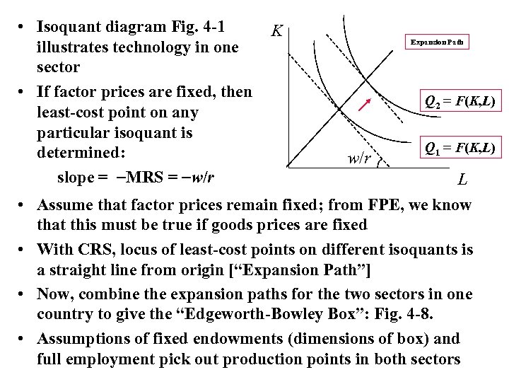• Isoquant diagram Fig. 4 -1 illustrates technology in one sector • If factor prices are fixed, then least-cost point on any particular isoquant is determined: slope = MRS = w/r • • K Expansion Path Q 2 = F(K, L) w/r Q 1 = F(K, L) L Assume that factor prices remain fixed; from FPE, we know that this must be true if goods prices are fixed With CRS, locus of least-cost points on different isoquants is a straight line from origin [“Expansion Path”] Now, combine the expansion paths for the two sectors in one country to give the “Edgeworth-Bowley Box”: Fig. 4 -8. Assumptions of fixed endowments (dimensions of box) and full employment pick out production points in both sectors

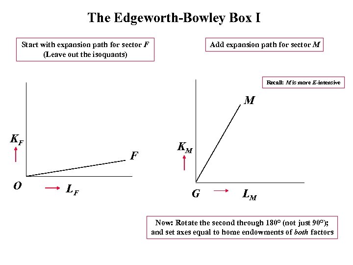The Edgeworth-Bowley Box I Start with expansion path for sector F (Leave out the isoquants) Add expansion path for sector M Recall: M is more K-intensive M KF F O LF KM G LM Now: Rotate the second through 180° (not just 90°); and set axes equal to home endowments of both factors

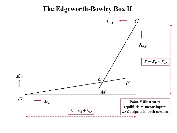The Edgeworth-Bowley Box II LM G KM K = KF + KM KF E F M O LF L = LF + LM Point E illustrates equilibrium factor inputs and outputs in both sectors

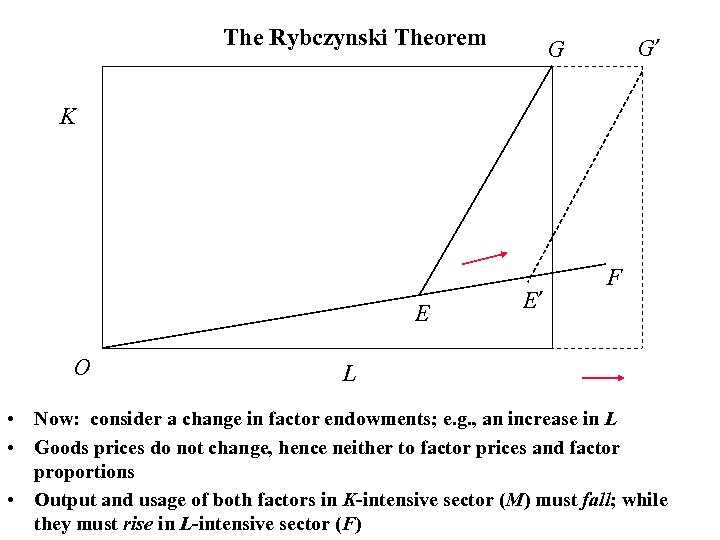The Rybczynski Theorem G’ G K E O E’ F L • Now: consider a change in factor endowments; e. g. , an increase in L • Goods prices do not change, hence neither to factor prices and factor proportions • Output and usage of both factors in K-intensive sector (M) must fall; while they must rise in L-intensive sector (F)

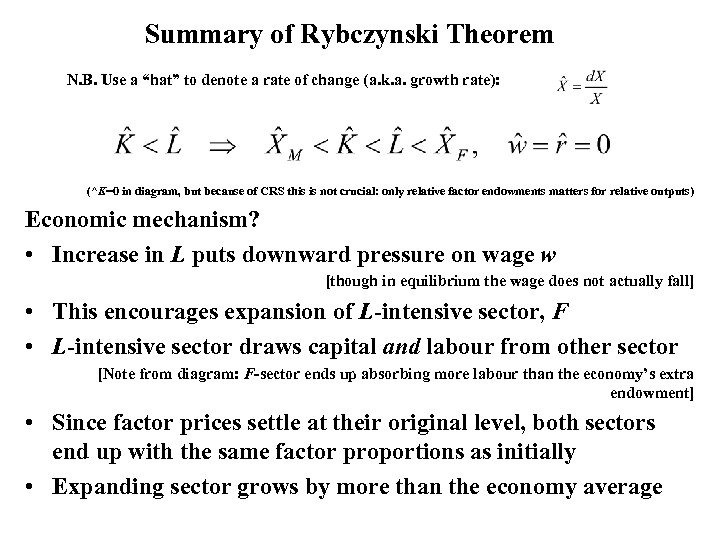Summary of Rybczynski Theorem N. B. Use a “hat” to denote a rate of change (a. k. a. growth rate): (^K=0 in diagram, but because of CRS this is not crucial: only relative factor endowments matters for relative outputs) Economic mechanism? • Increase in L puts downward pressure on wage w [though in equilibrium the wage does not actually fall] • This encourages expansion of L-intensive sector, F • L-intensive sector draws capital and labour from other sector [Note from diagram: F-sector ends up absorbing more labour than the economy’s extra endowment] • Since factor prices settle at their original level, both sectors end up with the same factor proportions as initially • Expanding sector grows by more than the economy average

Rybczynski Theorem (cont. ) Note: Theorem is very surprising - Economic growth occurs, yet output of one industry falls Basic idea: Source of growth is asymmetric; effect on pattern of outputs is even more asymmetric: asymmetry is magnified. Real-world examples? • Black Death in 13 th century Europe • Great Famine in Ireland, 1846 -49 • Russian emigration to Israel in 1990’s

Heckscher-Ohlin Theorem: A country has a comparative advantage in the good that uses relatively intensively the country’s relatively abundant factor Basically, extends the Rybczynski theorem from a time-series to a cross-section context, and neutralises the effects of demand differences between countries Steps in Proof: • Illustrate Rybczynski theorem in PPF diagram and reinterpret it in terms of a cross-section comparison between countries, which differ only in endowments of K (not L) • This shows that at the same prices, the more K-abundant country produces relatively more of the more K-intensive good. • Hence its relative supply curve (XM/XF) lies to right of the other country’s

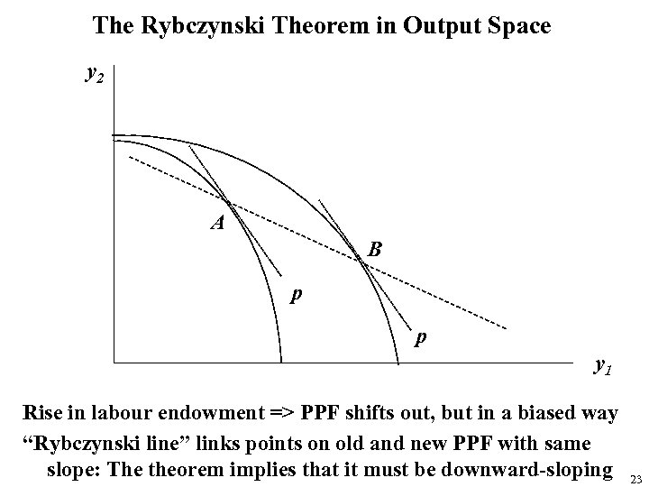The Rybczynski Theorem in Output Space y 2 A B p p y 1 Rise in labour endowment => PPF shifts out, but in a biased way “Rybczynski line” links points on old and new PPF with same slope: The theorem implies that it must be downward-sloping 23

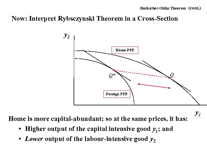Heckscher-Ohlin Theorem (cont. ) Now: Interpret Rybsczynski Theorem in a Cross-Section y 2 Home PPF Q* Q Foreign PPF Home is more capital-abundant; so at the same prices, it has: • Higher output of the capital intensive good y 1; and • Lower output of the labour-intensive good y 2 y 1

Heckscher-Ohlin Theorem (cont. ) Final step: Homothetic tastes • Imply that relative demands are the same at home and abroad • So: Production bias translates into a trade bias

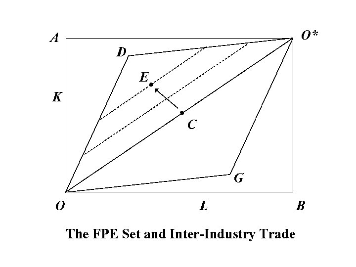A O* D E K C G O L The FPE Set and Inter-Industry Trade B