The Heckscher-Ohlin Model Appleyard Field Cobb

The Heckscher-Ohlin Model Appleyard & Field (& Cobb): Chapters 8 & 9 (Krugman & Obstfeld: Chapter 3 & 4) 1

Assumptions of the Heckscher-Ohlin(Samuelson)-Model 1. 2. 3. 4. 5. Two countries, two (homogeneous) goods and two (homogeneous) factors of production Identical technology, different factor endowments Constant returns to scale Different factor intensities in production Factors perfectly mobile inside each country and immobile between the countries 6. (Identical preferences among everyone) 7. Perfect competition in all markets → (price of labour) w = MPPL*P, (price of capital) r = MPPK*P 8. (No transportations costs) 2

Factor Endowments • Countries differ in their relative factor endowments • Notation: K=capital, L=labour, r = price of capital, w = price of labour • Physical definition: (K/L)1 > (K/L)2 country 1 is capital-abundant (labour-scarce), country 2 is labourabundant (capital-scarce) • Price definition: (r/w)1 < (r/w)2 country 1 is capital-abundant, country 2 is labour-abundant • Given assumptions of perfect competition + identical technology and preferences, the physical and price definitions are identical 3

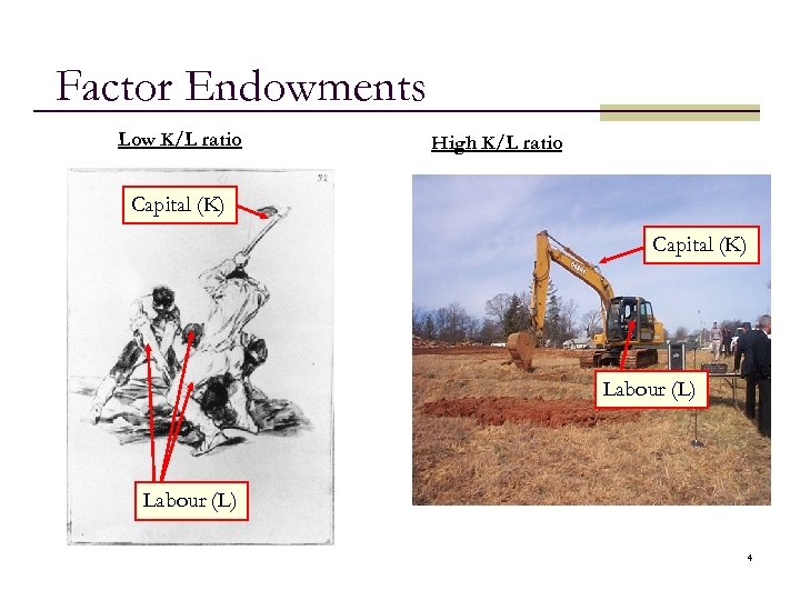
Factor Endowments Low K/L ratio High K/L ratio Capital (K) Labour (L) 4

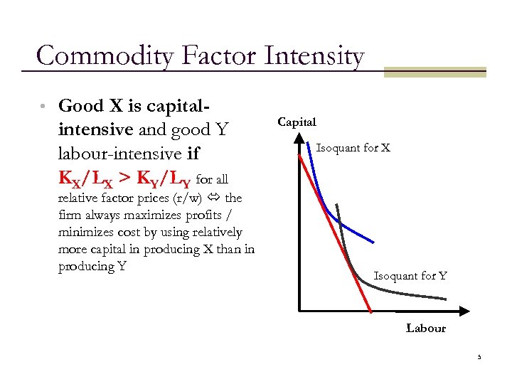
Commodity Factor Intensity • Good X is capital- intensive and good Y labour-intensive if KX/LX > KY/LY for all relative factor prices (r/w) the firm always maximizes profits / minimizes cost by using relatively more capital in producing X than in producing Y Capital Isoquant for X Isoquant for Y Labour 5

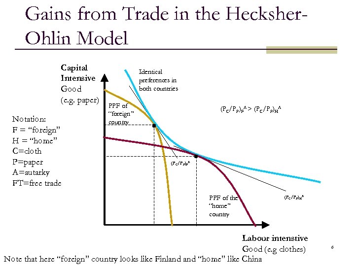
Gains from Trade in the Hecksher. Ohlin Model Capital Intensive Good (e. g. paper) Notation: F = “foreign” H = “home” C=cloth P=paper A=autarky FT=free trade Identical preferences in both countries PPF of “foreign” country (PC/PP)FA > (PC/PP)HA (PC/PP)FA PPF of the “home” country (PC/PP)HA Labour intenstive Good (e. g clothes) Note that here “foreign” country looks like Finland “home” like China 6

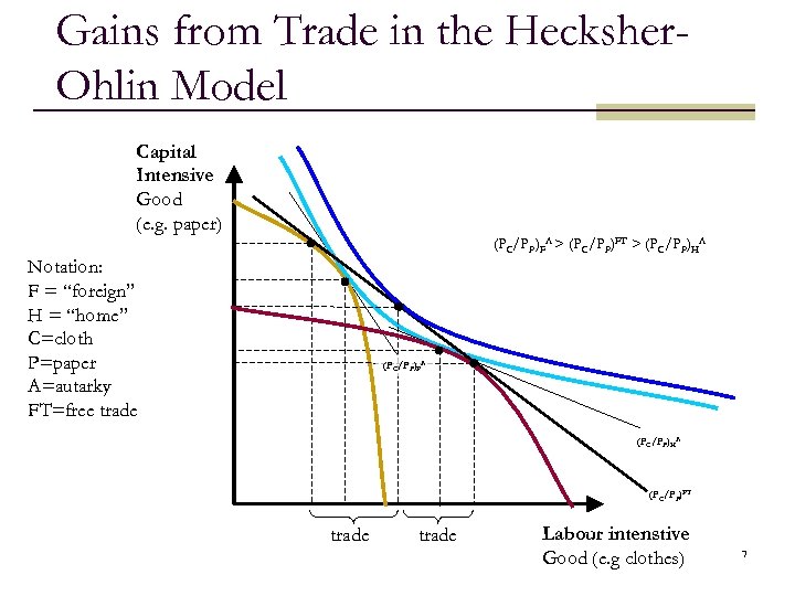
Gains from Trade in the Hecksher. Ohlin Model Capital Intensive Good (e. g. paper) (PC/PP)FA > (PC/PP)FT > (PC/PP)HA Notation: F = “foreign” H = “home” C=cloth P=paper A=autarky FT=free trade (PC/PP)FA (PC/PP)HA (PC/PP)FT trade Labour intenstive Good (e. g clothes) 7

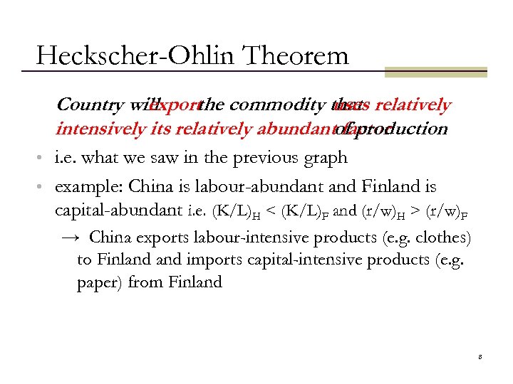
Heckscher-Ohlin Theorem Country will export commodity that relatively the uses intensively its relatively abundantof production factor • i. e. what we saw in the previous graph • example: China is labour-abundant and Finland is capital-abundant i. e. (K/L)H < (K/L)F and (r/w)H > (r/w)F → China exports labour-intensive products (e. g. clothes) to Finland imports capital-intensive products (e. g. paper) from Finland 8

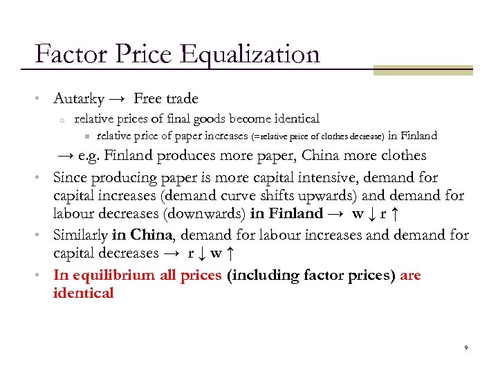
Factor Price Equalization • Autarky → Free trade o relative prices of final goods become identical n relative price of paper increases (=relative price of clothes decrease) in Finland → e. g. Finland produces more paper, China more clothes • Since producing paper is more capital intensive, demand for capital increases (demand curve shifts upwards) and demand for labour decreases (downwards) in Finland → w ↓ r ↑ • Similarly in China, demand for labour increases and demand for capital decreases → r ↓ w ↑ • In equilibrium all prices (including factor prices) are identical 9

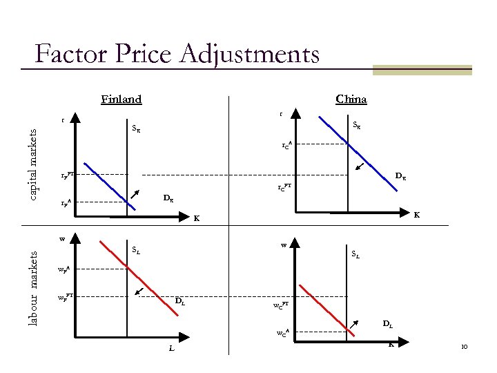
Factor Price Adjustments Finland capital markets r China r SK SK r. CA r. FFT DK r. CFT DK r. F A K K labour markets w w SL SL w. F A w. FFT DL w. CFT w. CA L DL K 10

Income Distribution and Trade: the Stolper-Samuelson Theorem • Trade affects both the prices of goods and the prices of factors of production: What then is the impact of trade on distribution of real income? o wages decrease in Finland, but also the price of clothes decreases (i. e. you need less money to buy the same amount of clothes). Which effect dominates? • Stolper-Samuelson Theorem: real income of the owners of abundant factor increases and the real income of owners of scarce factor decreases o Think about the labour abundant country (e. g. China): Free trade → r ↓ w ↑ → capital/labour ratio ↑ → labour productivity ↑ → real wages ↑ 11 W. Stolper & P. Samuelson (1941): International Factor-Price Equalisation Once Again. Economic Journal 59, no. 234.

Why Don’t We Observe Price Equalization? • In reality most of the assumptions needed for price equalization do not hold o e. g. differences in productivity / technology, transportation costs, tariffs, subsidies, imperfect competition, unemployed resources, externalities… • However, the model provides an important insight on the tendency of price movements due to increasing international trade 12

Trade as a Substitute for Capital and Labour Flows • Suppose that there is no international trade of goods, but capital and labour are internationally perfectly mobile • Capital will then flow to the labour-abundant country and labour to the capital-abundant country until the factor prices are equal in both countries • When all markets are perfectly competitive, this must imply equal commodity prices → Trade and factor mobility are perfect substitutes in the HO-model 13 R. A. Mundell (1957): International Trade and Factor Mobility. American Economic Review 47(3).

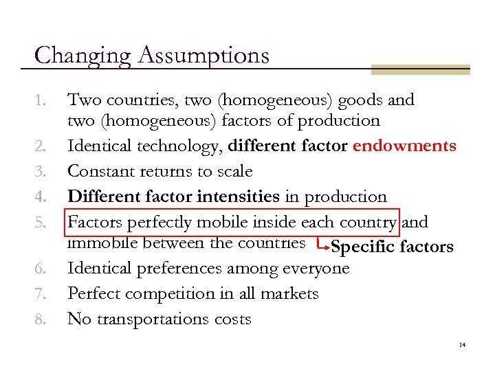
Changing Assumptions 1. 2. 3. 4. 5. 6. 7. 8. Two countries, two (homogeneous) goods and two (homogeneous) factors of production Identical technology, different factor endowments Constant returns to scale Different factor intensities in production Factors perfectly mobile inside each country and immobile between the countries Specific factors Identical preferences among everyone Perfect competition in all markets No transportations costs 14

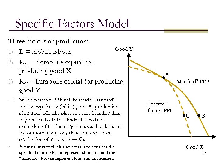
Specific-Factors Model Three factors of production: Good Y 1) L = mobile labour 2) KX = immobile capital for producing good X 3) KY = immobile capital for producing good Y → Specific-factors PPF will lie inside “standard” PPF, except in the (initial) point A (production after trade will take place in point C, rather than in point B). Note that trade still leads to expansion of the industry that uses the abundant factor more intensively (labour moves from production of Y to X; A → C). o A natural way to think about this is to consider the specific-factors PPF to represent short-run and the “standard” PPF to represent long-run implications A “standard” PPF Specificfactors PPF C B Good X 15

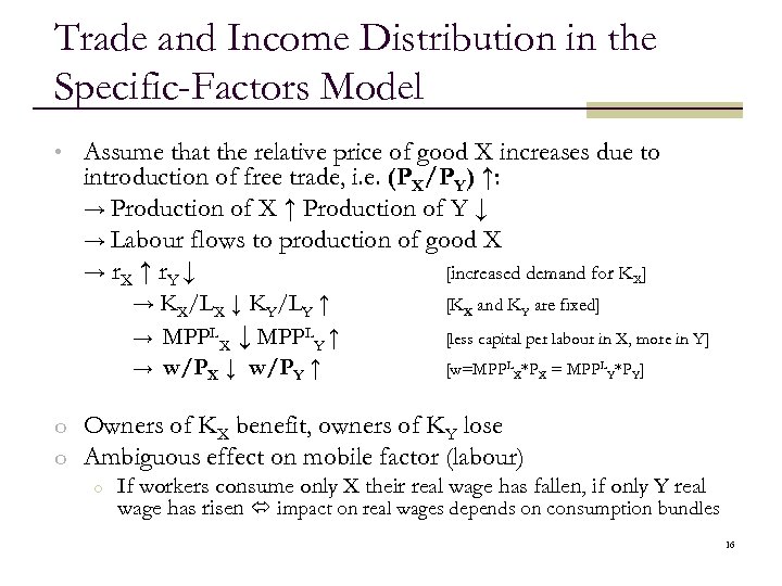
Trade and Income Distribution in the Specific-Factors Model • Assume that the relative price of good X increases due to introduction of free trade, i. e. (PX/PY) ↑: → Production of X ↑ Production of Y ↓ → Labour flows to production of good X → r. X ↑ r. Y ↓ [increased demand for KX] → KX/LX ↓ KY/LY ↑ → MPPLX ↓ MPPLY ↑ → w/PX ↓ w/PY ↑ [KX and KY are fixed] [less capital per labour in X, more in Y] [w=MPPLX*PX = MPPLY*PY] o Owners of KX benefit, owners of KY lose o Ambiguous effect on mobile factor (labour) o If workers consume only X their real wage has fallen, if only Y real wage has risen impact on real wages depends on consumption bundles 16

Summary of the Heckscher-Ohlin model • Differences in relative endowments of factors of production → Comparative advantage • Trade leads to o o Expansion of the industry using intensively the abundant factor of production (Heckscher-Ohlin Theorem) Changes in distribution of income (international factor price equalization, Stolper-Samuelson theorem) 17

Is trade beneficial in the HO-Model? • We have seen that trade benefits some* and hurts others**. So, • • do the gains outweigh the losses? To answer this question would require comparison of (subjective) welfares (do the losers suffer more than the winners enjoy), which is outside of the province of economic analysis. However, we can ask: Could those who gain compensate those who lose, and still be better off? The answer is, yes. Trade expands the economy’s choices (enables consumption outside PPF). Hence, in principle, it is possible to redistribute income in such a way that everyone will gain. Of course, this is not to say that redistribution would actually happen. The presence of loser and winners in the real world is probably the most important reason why trade is not free. 18 * owners of the abundant / export specific factor; ** owners of the scarce / import specific factor