8c637ad4c55fce4d499fde1a01967cc2.ppt
- Количество слайдов: 78
The Future of Numerical Linear Algebra Automatic Performance Tuning of Sparse Matrix codes The Next LAPACK and Sca. LAPACK www. cs. berkeley. edu/~demmel/Utah_Apr 05. ppt James Demmel UC Berkeley
Outline • Automatic Performance Tuning of Sparse Matrix Kernels • Updating LAPACK and Sca. LAPACK
Outline • Automatic Performance Tuning of Sparse Matrix Kernels • Updating LAPACK and Sca. LAPACK
Berkeley Benchmarking and OPtimization (Be. BOP) • Prof. Katherine Yelick • Rich Vuduc – Many results in this talk are from Vuduc’s Ph. D thesis, www. cs. berkeley. edu/~richie • Rajesh Nishtala, Mark Hoemmen, Hormozd Gahvari • Eun-Jim Im, many other earlier contributors • Other papers at bebop. cs. berkeley. edu

Motivation for Automatic Performance Tuning • Writing high performance software is hard – Make programming easier while getting high speed • Ideal: program in your favorite high level language (Matlab, PETSc…) and get a high fraction of peak performance • Reality: Best algorithm (and its implementation) can depend strongly on the problem, computer architecture, compiler, … – Best choice can depend on knowing a lot of applied mathematics and computer science • How much of this can we teach?
Motivation for Automatic Performance Tuning • Writing high performance software is hard – Make programming easier while getting high speed • Ideal: program in your favorite high level language (Matlab, PETSc…) and get a high fraction of peak performance • Reality: Best algorithm (and its implementation) can depend strongly on the problem, computer architecture, compiler, … – Best choice can depend on knowing a lot of applied mathematics and computer science • How much of this can we teach? • How much of this can we automate?
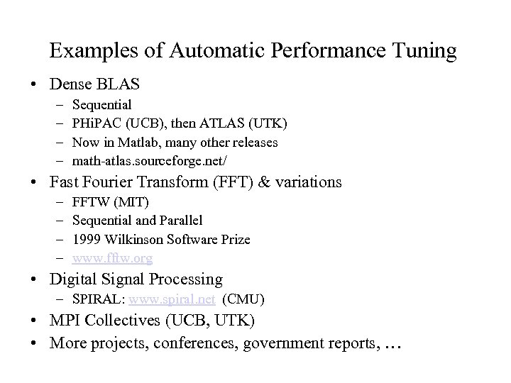
Examples of Automatic Performance Tuning • Dense BLAS – – Sequential PHi. PAC (UCB), then ATLAS (UTK) Now in Matlab, many other releases math-atlas. sourceforge. net/ • Fast Fourier Transform (FFT) & variations – – FFTW (MIT) Sequential and Parallel 1999 Wilkinson Software Prize www. fftw. org • Digital Signal Processing – SPIRAL: www. spiral. net (CMU) • MPI Collectives (UCB, UTK) • More projects, conferences, government reports, …
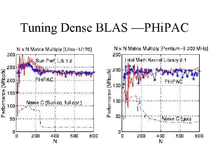
Tuning Dense BLAS —PHi. PAC
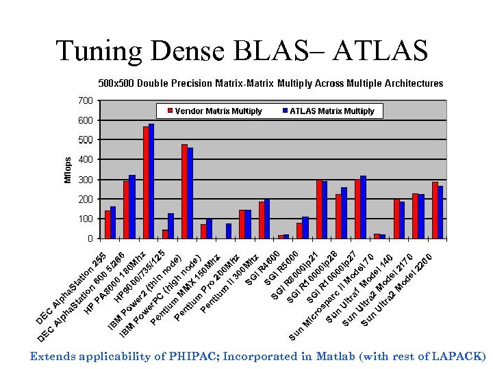
Tuning Dense BLAS– ATLAS Extends applicability of PHIPAC; Incorporated in Matlab (with rest of LAPACK)
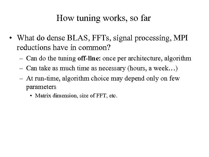
How tuning works, so far • What do dense BLAS, FFTs, signal processing, MPI reductions have in common? – Can do the tuning off-line: once per architecture, algorithm – Can take as much time as necessary (hours, a week…) – At run-time, algorithm choice may depend only on few parameters • Matrix dimension, size of FFT, etc.
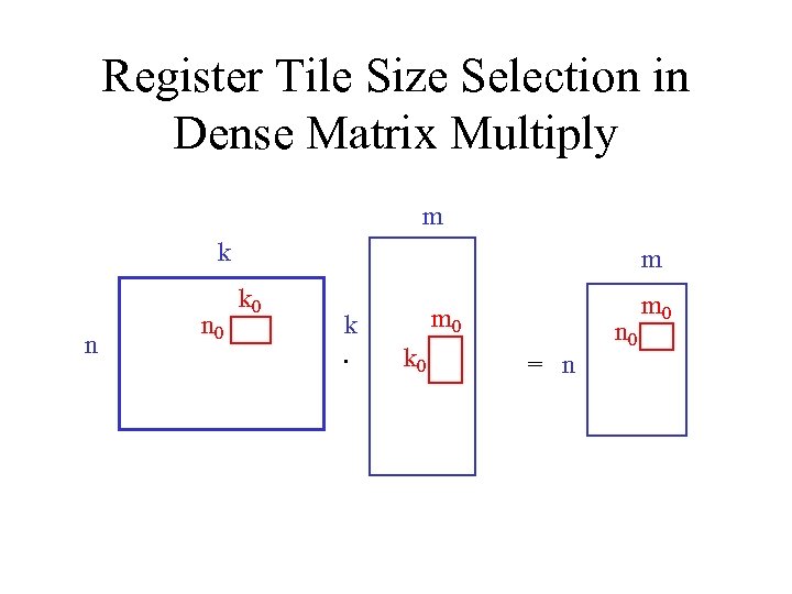
Register Tile Size Selection in Dense Matrix Multiply m k n n 0 m k 0 k. m 0 k 0 n 0 = n m 0
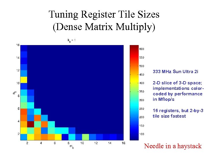
Tuning Register Tile Sizes (Dense Matrix Multiply) 333 MHz Sun Ultra 2 i 2 -D slice of 3 -D space; implementations colorcoded by performance in Mflop/s 16 registers, but 2 -by-3 tile size fastest Needle in a haystack
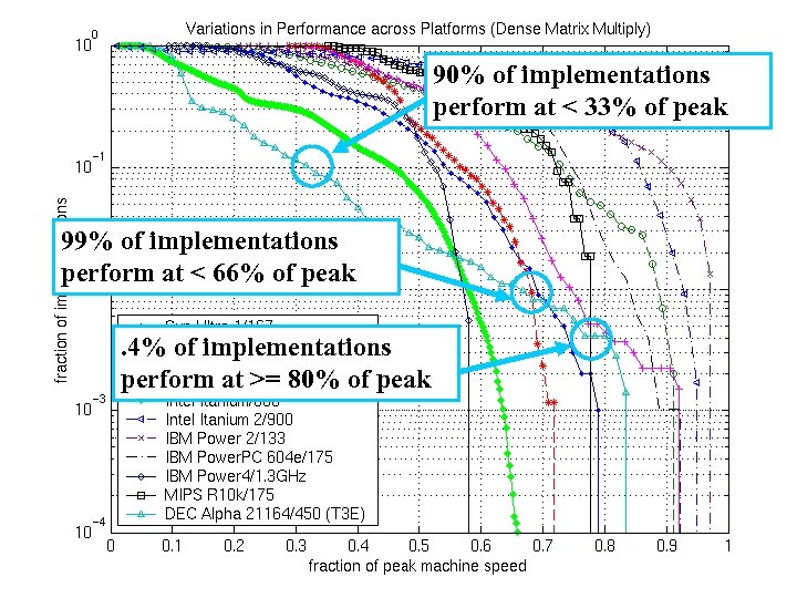
90% of implementations perform at < 33% of peak 99% of implementations perform at < 66% of peak. 4% of implementations perform at >= 80% of peak
Limits of off-line tuning • Algorithm and its implementation may strongly depend on data only known at run-time • Ex: Sparse matrix nonzero pattern determines both best data structure and implementation of Sparse-matrix-vector-multiplication (Sp. MV) • Can’t afford to generate and test thousands of algorithms and implementations at run-time! • BEBOP project addresses sparse tuning
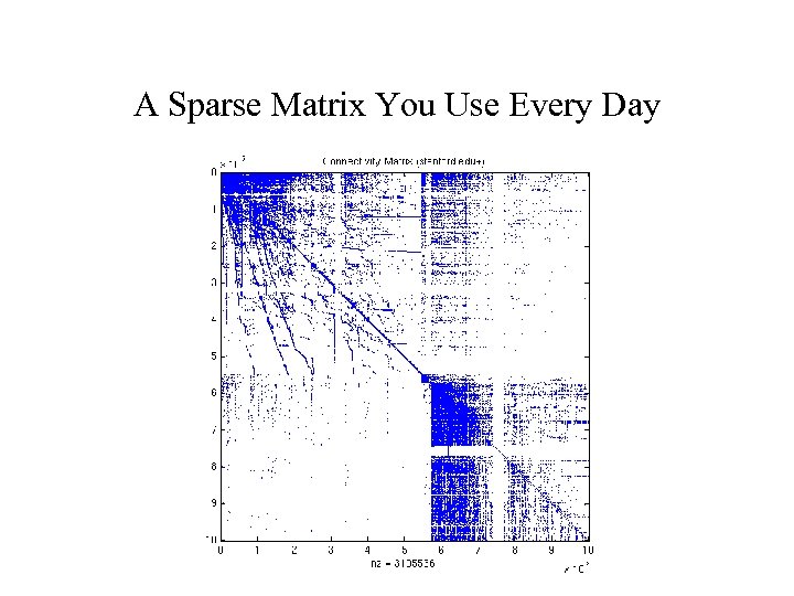
A Sparse Matrix You Use Every Day
Motivation for Automatic Performance Tuning of Sp. MV • Sp. MV widely used in practice – Kernel of iterative solvers for • linear systems • eigenvalue problems • Singular value problems • Historical trends – Sparse matrix-vector multiply (Sp. MV): 10% of peak or less – 2 x faster than CSR with “hand-tuning” – Tuning becoming more difficult over time
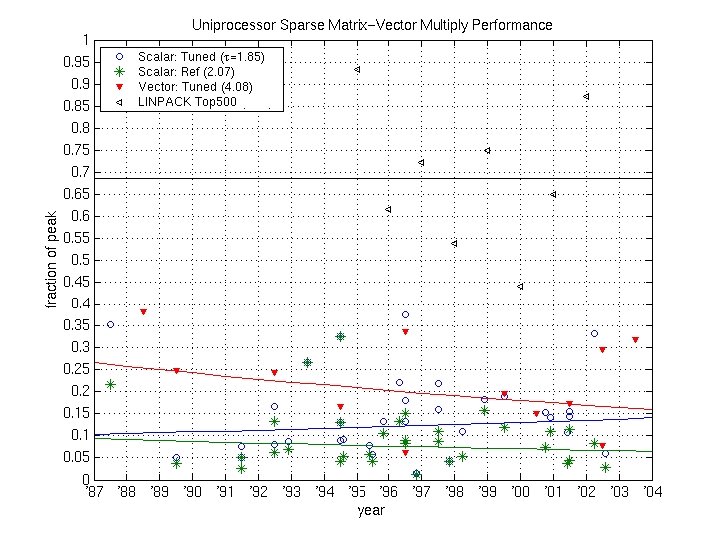
Sp. MV Historical Trends: Fraction of Peak
Approach to Automatic Performance Tuning of Sp. MV • Our approach: empirical modeling and search – Off-line: measure performance of variety of data structures and Sp. MV algorithms – On-line: sample matrix, use performance model to predict which data structure/algorithm is best • Results – Up to 4 x speedups and 31% of peak for Sp. MV • Using register blocking – Many other optimization techniques for Sp. MV
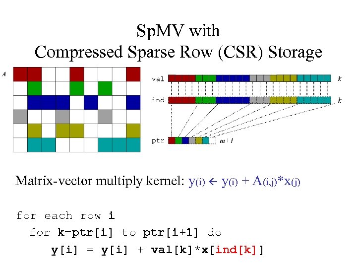
Sp. MV with Compressed Sparse Row (CSR) Storage Matrix-vector multiply kernel: y(i) + A(i, j)*x(j) for each row i for k=ptr[i] to ptr[i+1] do y[i] = y[i] + val[k]*x[ind[k]]
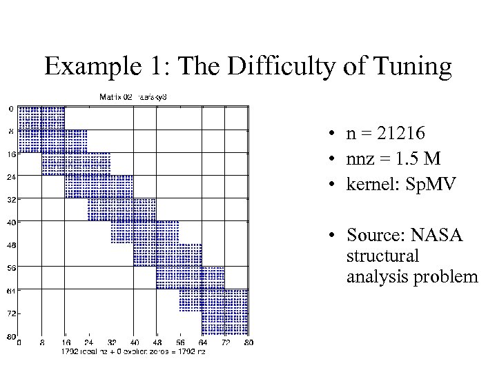
Example 1: The Difficulty of Tuning • n = 21216 • nnz = 1. 5 M • kernel: Sp. MV • Source: NASA structural analysis problem
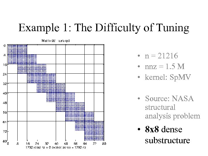
Example 1: The Difficulty of Tuning • n = 21216 • nnz = 1. 5 M • kernel: Sp. MV • Source: NASA structural analysis problem • 8 x 8 dense substructure
Taking advantage of block structure in Sp. MV • Bottleneck is time to get matrix from memory – Only 2 flops for each nonzero in matrix – Goal: decrease size of data structure • Don’t store each nonzero with index, instead store each nonzero r-by-c block with one index – Storage drops by up to 2 x (if rc >> 1, all 32 -bit quantities) – Time to fetch matrix from memory decreases • Change both data structure and algorithm – Need to pick r and c – Need to change algorithm accordingly • In example, is r=c=8 best choice? – Minimizes storage, so looks like a good idea…
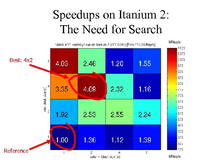
Speedups on Itanium 2: The Need for Search Mflop/s Best: 4 x 2 Reference Mflop/s
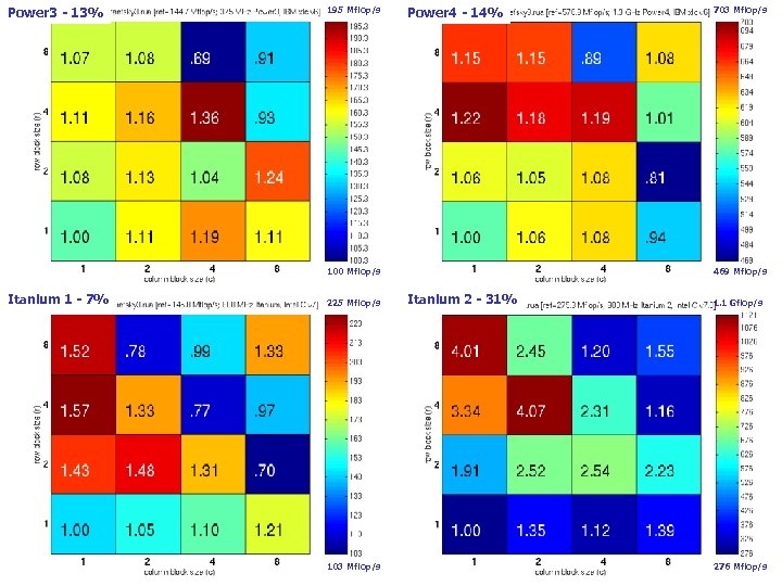
Power 3 - 13% 195 Mflop/s Power 4 - 14% 703 Mflop/s Sp. MV Performance (Matrix #2): Generation 1 100 Mflop/s Itanium 1 - 7% 225 Mflop/s 103 Mflop/s 469 Mflop/s Itanium 2 - 31% 1. 1 Gflop/s 276 Mflop/s
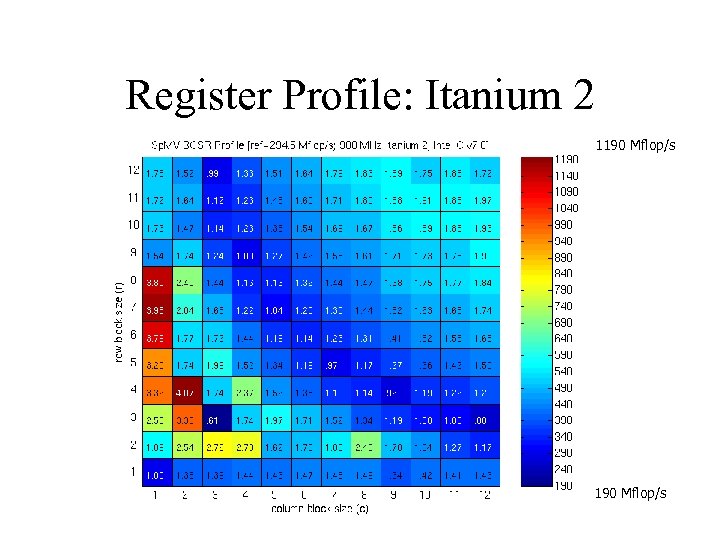
Register Profile: Itanium 2 1190 Mflop/s
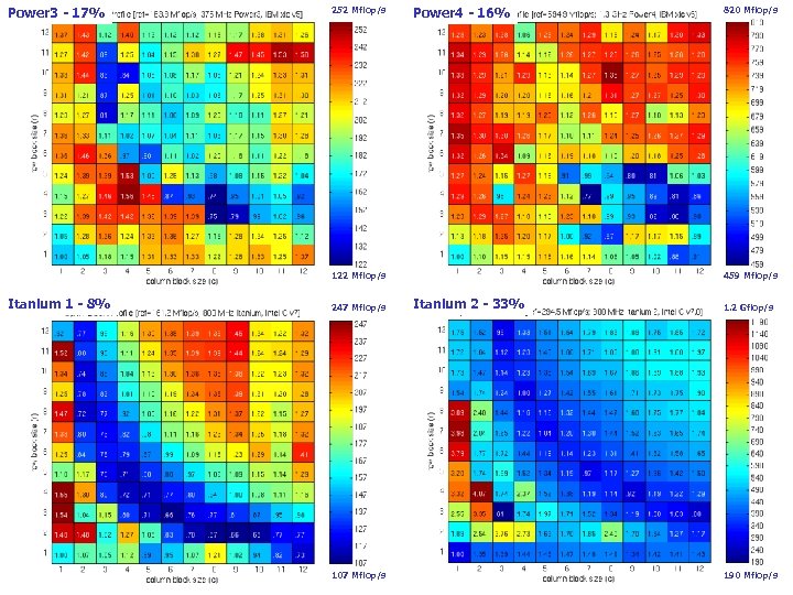
Power 3 - 17% 252 Mflop/s Power 4 - 16% 820 Mflop/s Register Profiles: IBM and Intel IA-64 122 Mflop/s Itanium 1 - 8% 247 Mflop/s 107 Mflop/s 459 Mflop/s Itanium 2 - 33% 1. 2 Gflop/s 190 Mflop/s
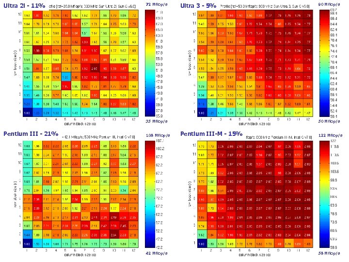
Ultra 2 i - 11% 72 Mflop/s Ultra 3 - 5% 90 Mflop/s Register Profiles: Sun and Intel x 86 35 Mflop/s Pentium III - 21% 108 Mflop/s 42 Mflop/s 50 Mflop/s Pentium III-M - 15% 122 Mflop/s 58 Mflop/s
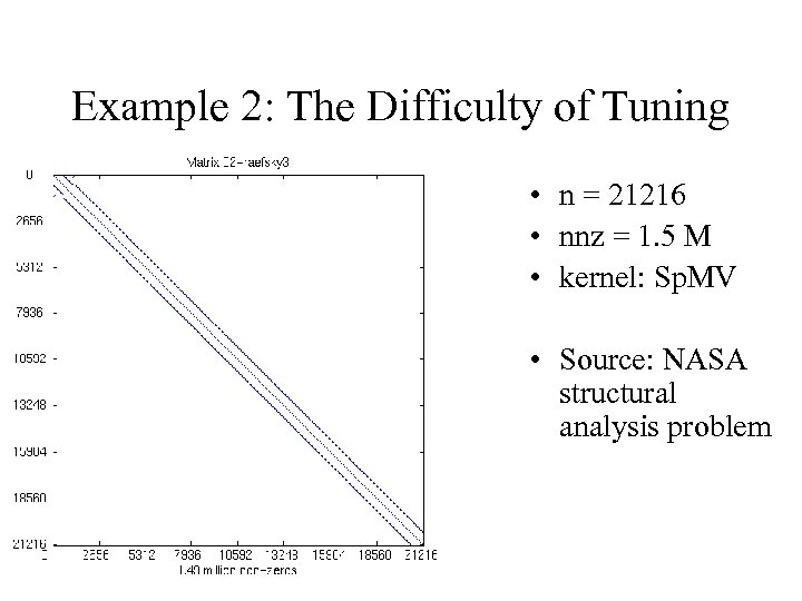
Example 2: The Difficulty of Tuning • n = 21216 • nnz = 1. 5 M • kernel: Sp. MV • Source: NASA structural analysis problem
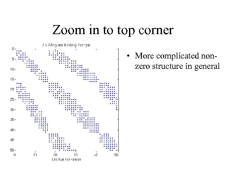
Zoom in to top corner • More complicated nonzero structure in general
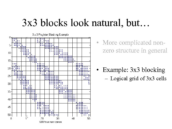
3 x 3 blocks look natural, but… • More complicated nonzero structure in general • Example: 3 x 3 blocking – Logical grid of 3 x 3 cells
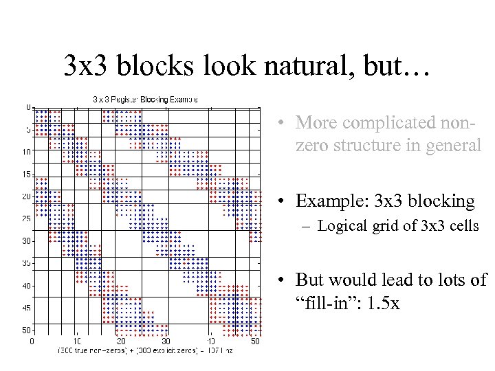
3 x 3 blocks look natural, but… • More complicated nonzero structure in general • Example: 3 x 3 blocking – Logical grid of 3 x 3 cells • But would lead to lots of “fill-in”: 1. 5 x
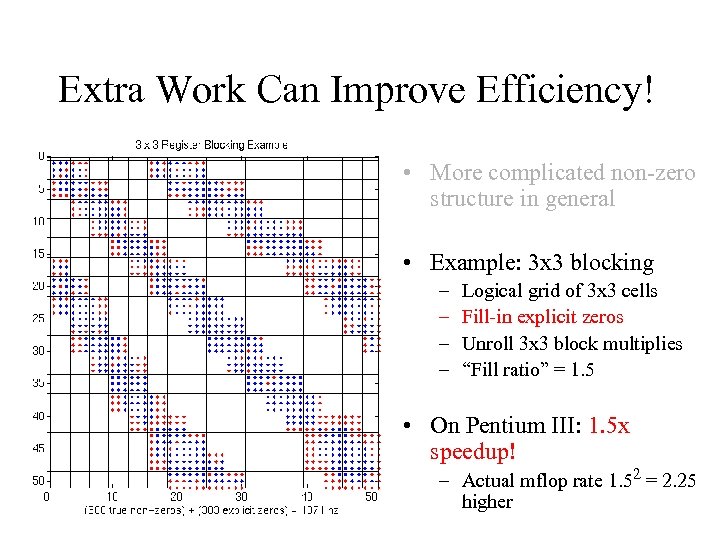
Extra Work Can Improve Efficiency! • More complicated non-zero structure in general • Example: 3 x 3 blocking – – Logical grid of 3 x 3 cells Fill-in explicit zeros Unroll 3 x 3 block multiplies “Fill ratio” = 1. 5 • On Pentium III: 1. 5 x speedup! – Actual mflop rate 1. 52 = 2. 25 higher
Automatic Register Block Size Selection • Selecting the r x c block size – Off-line benchmark • Precompute Mflops(r, c) using dense A for each r x c • Once per machine/architecture – Run-time “search” • Sample A to estimate Fill(r, c) for each r x c – Run-time heuristic model • Choose r, c to minimize time Fill(r, c) / Mflops(r, c)
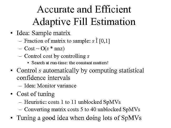
Accurate and Efficient Adaptive Fill Estimation • Idea: Sample matrix – Fraction of matrix to sample: s Î [0, 1] – Cost ~ O(s * nnz) – Control cost by controlling s • Search at run-time: the constant matters! • Control s automatically by computing statistical confidence intervals – Idea: Monitor variance • Cost of tuning – Heuristic: costs 1 to 11 unblocked Sp. MVs – Converting matrix costs 5 to 40 unblocked Sp. MVs • Tuning a good idea when doing lots of Sp. MVs
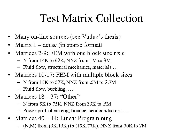
Test Matrix Collection • Many on-line sources (see Vuduc’s thesis) • Matrix 1 – dense (in sparse format) • Matrices 2 -9: FEM with one block size r x c – N from 14 K to 62 K, NNZ from 1 M to 3 M – Fluid flow, structural mechanics, materials … • Matrices 10 -17: FEM with multiple block sizes – N from 17 K to 52 K, NNZ from. 5 M to 2. 7 M – Fluid flow, buckling, … • Matrices 18 – 37: “Other” – N from 5 K to 75 K, NNZ from 33 K to. 5 M – Power grid, chem eng, finance, semiconductors, … • Matrices 40 – 44: Linear Programming – (N, M) from (3 K, 13 K) to (15 K, 77 K), NNZ from 50 K to 2 M
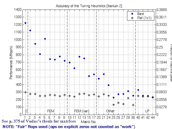
Accuracy of the Tuning Heuristics (1/4) See p. 375 of Vuduc’s thesis for matrices NOTE: “Fair” flops used (ops on explicit zeros not counted as “work”)
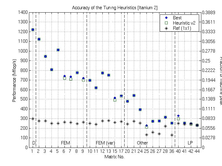
Accuracy of the Tuning Heuristics (2/4)
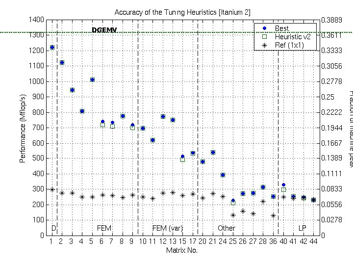
Accuracy of the Tuning Heuristics (2/4) DGEMV

Evaluating algorithms and machines for Sp. MV • Some speedups look good, but could we do better? • Questions – What is the best speedup possible? • Independent of instruction scheduling, selection • Can Sp. MV be further improved or not? – What machines are “good” for Sp. MV? – How can architectures be changed to improve Sp. MV?
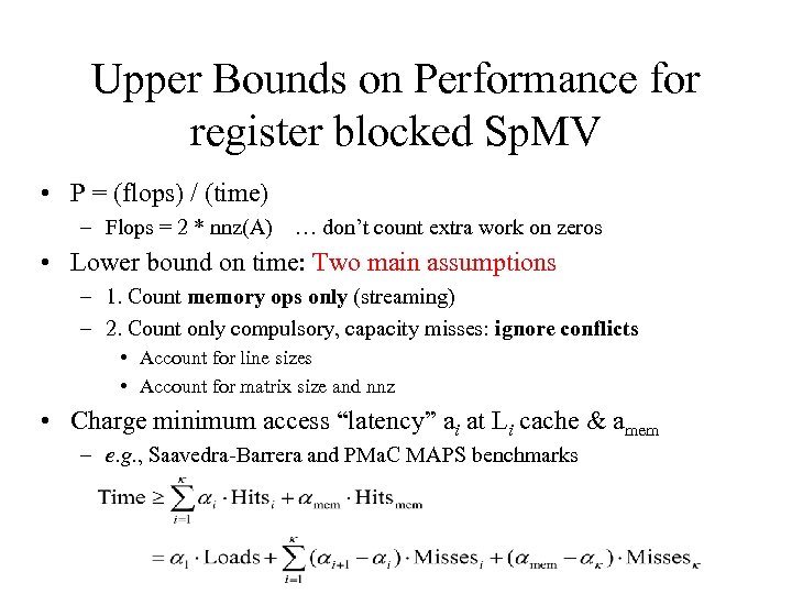
Upper Bounds on Performance for register blocked Sp. MV • P = (flops) / (time) – Flops = 2 * nnz(A) … don’t count extra work on zeros • Lower bound on time: Two main assumptions – 1. Count memory ops only (streaming) – 2. Count only compulsory, capacity misses: ignore conflicts • Account for line sizes • Account for matrix size and nnz • Charge minimum access “latency” ai at Li cache & amem – e. g. , Saavedra-Barrera and PMa. C MAPS benchmarks
![Example: L 2 Misses on Itanium 2 Misses measured using PAPI [Browne ’ 00] Example: L 2 Misses on Itanium 2 Misses measured using PAPI [Browne ’ 00]](https://present5.com/presentation/8c637ad4c55fce4d499fde1a01967cc2/image-41.jpg)
Example: L 2 Misses on Itanium 2 Misses measured using PAPI [Browne ’ 00]
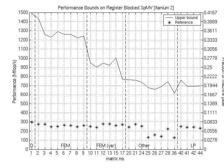
Example: Bounds on Itanium 2
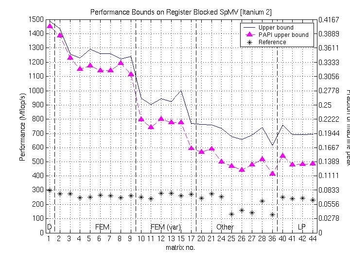
Example: Bounds on Itanium 2
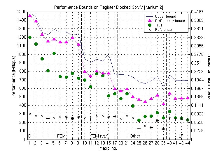
Example: Bounds on Itanium 2
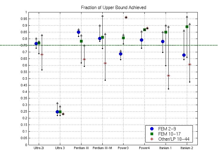
Fraction of Upper Bound Across Platforms
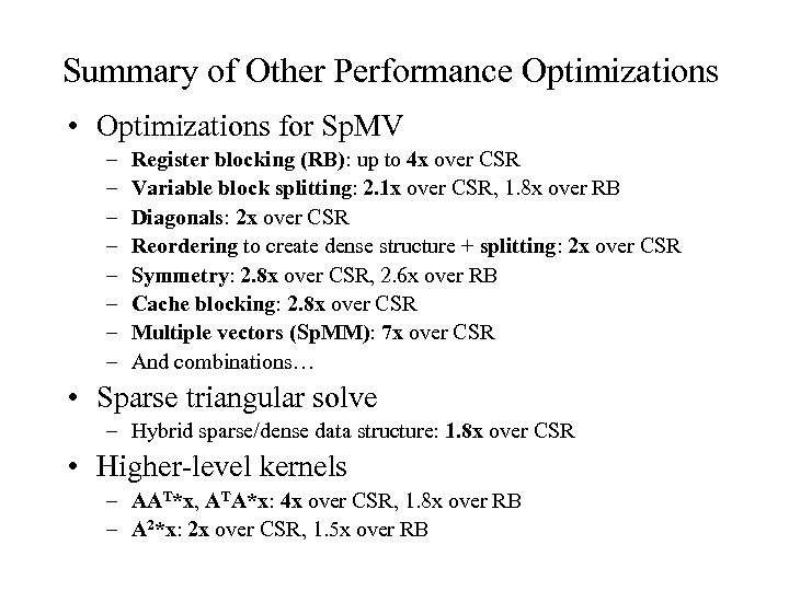
Summary of Other Performance Optimizations • Optimizations for Sp. MV – – – – Register blocking (RB): up to 4 x over CSR Variable block splitting: 2. 1 x over CSR, 1. 8 x over RB Diagonals: 2 x over CSR Reordering to create dense structure + splitting: 2 x over CSR Symmetry: 2. 8 x over CSR, 2. 6 x over RB Cache blocking: 2. 8 x over CSR Multiple vectors (Sp. MM): 7 x over CSR And combinations… • Sparse triangular solve – Hybrid sparse/dense data structure: 1. 8 x over CSR • Higher-level kernels – AAT*x, ATA*x: 4 x over CSR, 1. 8 x over RB – A 2*x: 2 x over CSR, 1. 5 x over RB
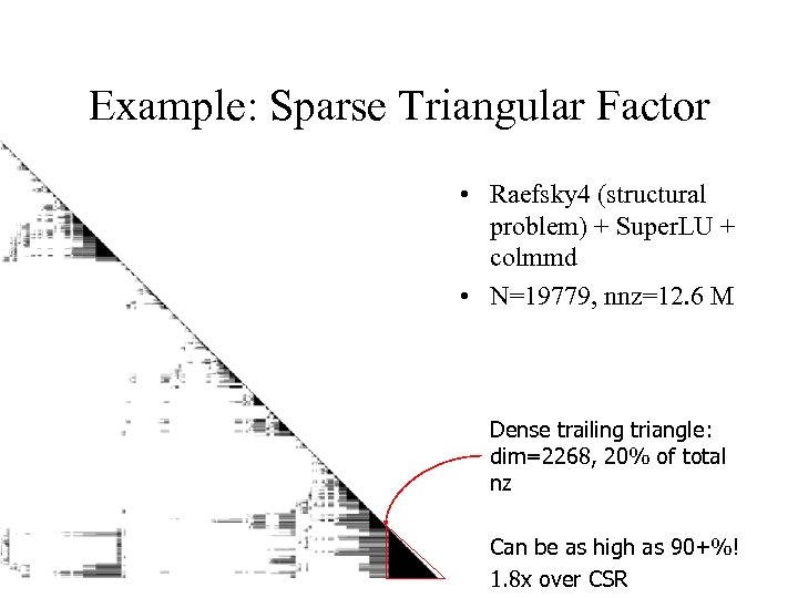
Example: Sparse Triangular Factor • Raefsky 4 (structural problem) + Super. LU + colmmd • N=19779, nnz=12. 6 M Dense trailing triangle: dim=2268, 20% of total nz Can be as high as 90+%! 1. 8 x over CSR
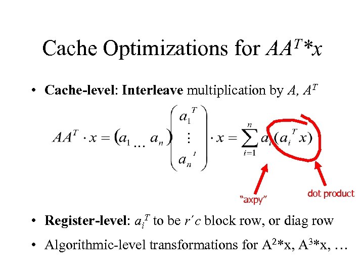
Cache Optimizations for T*x AA … … • Cache-level: Interleave multiplication by A, AT “axpy” dot product • Register-level: ai. T to be r´c block row, or diag row • Algorithmic-level transformations for A 2*x, A 3*x, …
![Impact on Applications: Omega 3 P • Application: accelerator cavity design [Ko] • Relevant Impact on Applications: Omega 3 P • Application: accelerator cavity design [Ko] • Relevant](https://present5.com/presentation/8c637ad4c55fce4d499fde1a01967cc2/image-49.jpg)
Impact on Applications: Omega 3 P • Application: accelerator cavity design [Ko] • Relevant optimization techniques – Symmetric storage – Register blocking – Reordering rows and columns to improve blocking • Reverse Cuthill-Mc. Kee ordering to reduce bandwidth • Traveling Salesman Problem-based ordering to create blocks – [Pinar & Heath ’ 97] – Make columns adjacent if they have many common nonzero rows • 2. 1 x speedup on Power 4
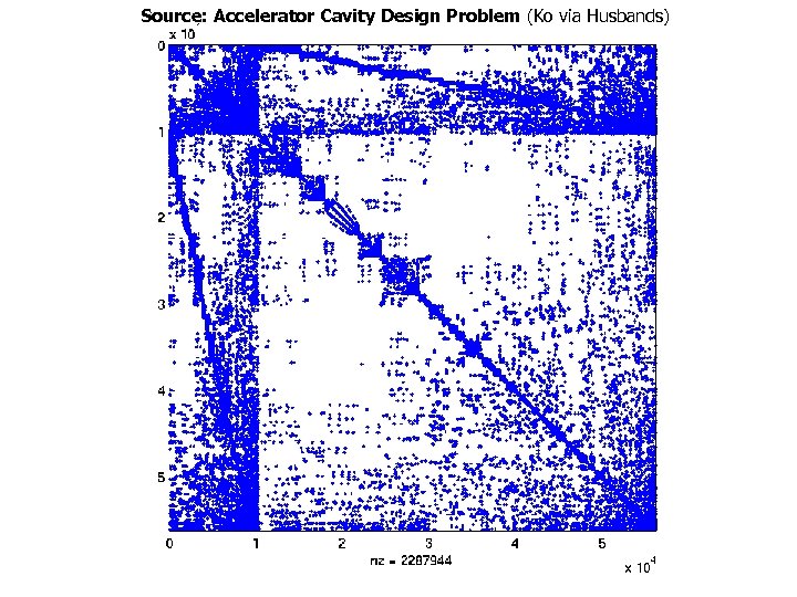
Source: Accelerator Cavity Design Problem (Ko via Husbands)
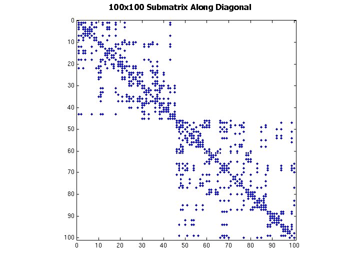
100 x 100 Submatrix Along Diagonal
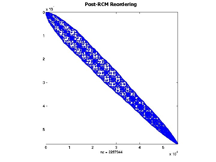
Post-RCM Reordering
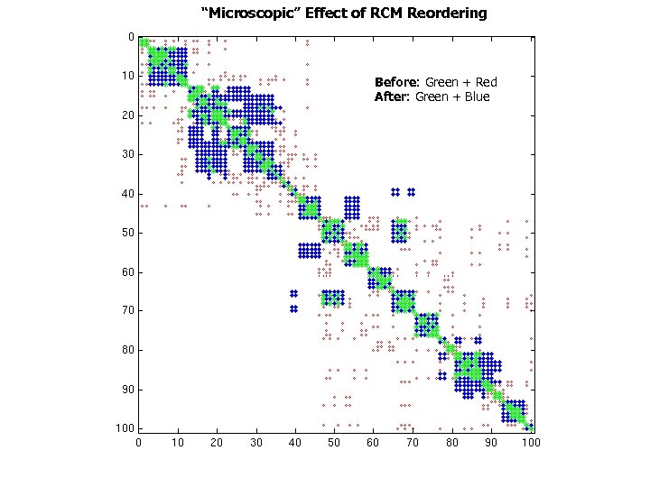
“Microscopic” Effect of RCM Reordering Before: Green + Red After: Green + Blue
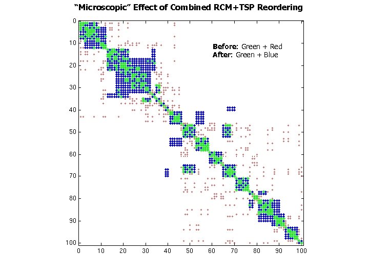
“Microscopic” Effect of Combined RCM+TSP Reordering Before: Green + Red After: Green + Blue
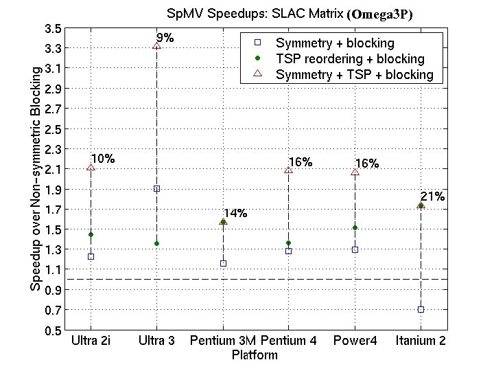
(Omega 3 P)
Optimized Sparse Kernel Interface OSKI • Provides sparse kernels automatically tuned for user’s matrix & machine – BLAS-style functionality: Sp. MV, Ax & ATy, Tr. SV – Hides complexity of run-time tuning – Includes ATAx, Akx • For “advanced” users & solver library writers – Available as stand-alone library • Alpha release at bebop. cs. berkeley. edu/oski • Release v 1. 0 “soon” – Will be available as PETSc extension See: bebop. cs. berkeley. edu
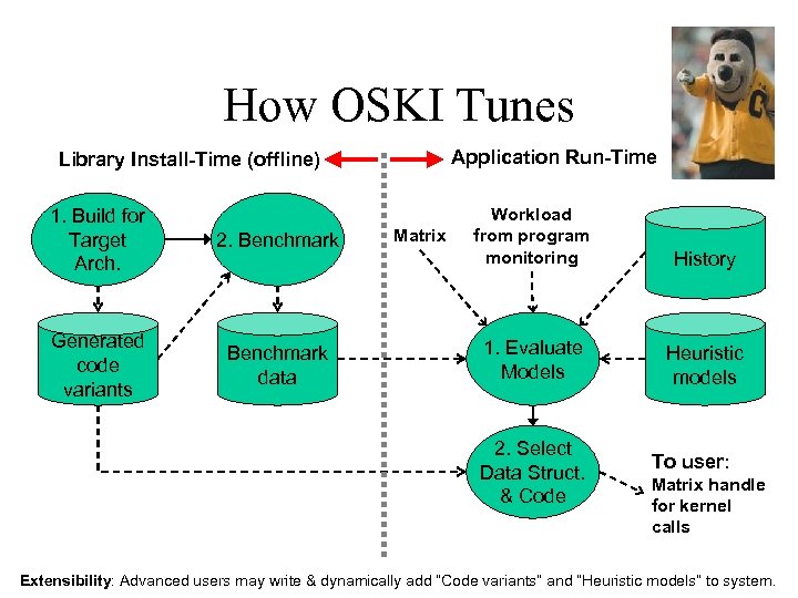
How OSKI Tunes Application Run-Time Library Install-Time (offline) 1. Build for Target Arch. 2. Benchmark Generated code variants Benchmark data Matrix Workload from program monitoring History 1. Evaluate Models Heuristic models 2. Select Data Struct. & Code To user: Matrix handle for kernel calls Extensibility: Advanced users may write & dynamically add “Code variants” and “Heuristic models” to system.
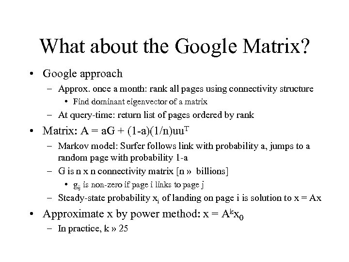
What about the Google Matrix? • Google approach – Approx. once a month: rank all pages using connectivity structure • Find dominant eigenvector of a matrix – At query-time: return list of pages ordered by rank • Matrix: A = a. G + (1 -a)(1/n)uu. T – Markov model: Surfer follows link with probability a, jumps to a random page with probability 1 -a – G is n x n connectivity matrix [n » billions] • gij is non-zero if page i links to page j – Steady-state probability xi of landing on page i is solution to x = Ax • Approximate x by power method: x = Akx 0 – In practice, k » 25
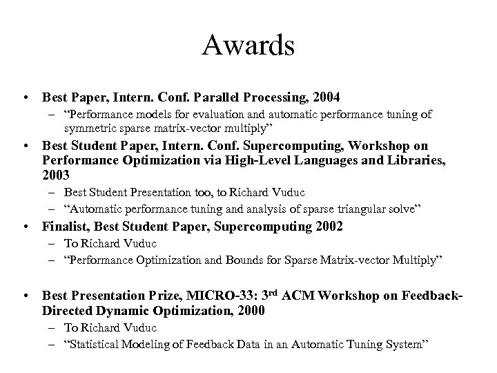
Awards • Best Paper, Intern. Conf. Parallel Processing, 2004 – “Performance models for evaluation and automatic performance tuning of symmetric sparse matrix-vector multiply” • Best Student Paper, Intern. Conf. Supercomputing, Workshop on Performance Optimization via High-Level Languages and Libraries, 2003 – Best Student Presentation too, to Richard Vuduc – “Automatic performance tuning and analysis of sparse triangular solve” • Finalist, Best Student Paper, Supercomputing 2002 – To Richard Vuduc – “Performance Optimization and Bounds for Sparse Matrix-vector Multiply” • Best Presentation Prize, MICRO-33: 3 rd ACM Workshop on Feedback. Directed Dynamic Optimization, 2000 – To Richard Vuduc – “Statistical Modeling of Feedback Data in an Automatic Tuning System”
Outline • Automatic Performance Tuning of Sparse Matrix Kernels • Updating LAPACK and Sca. LAPACK
LAPACK and Sca. LAPACK • Widely used dense and banded linear algebra libraries – In Matlab (thanks to tuning…), NAG, PETSc, … – Used in vendor libraries from Cray, Fujitsu, HP, IBM, Intel, NEC, SGI – over 49 M web hits at www. netlib. org • New NSF grant for new, improved releases – Joint with Jack Dongarra, many others – Community effort (academic and industry) – www. cs. berkeley. edu/~demmel/Sca-LAPACK-Proposal. pdf
Goals (highlights) • Putting more of LAPACK into Sca. LAPACK – Lots of routines not yet parallelized • New functionality – Ex: Updating/downdating of factorizations • Improving ease of use – Life after F 77? • Automatic Performance Tuning – Over 1300 calls to ILAENV() to get tuning parameters • New Algorithms – Some faster, some more accurate, some new
Faster: eig() and svd() • Nonsymmetric eigenproblem – Incorporate SIAM Prize winning work of Byers / Braman / Mathias on faster HQR – Up to 10 x faster for large enough problems • Symmetric eigenproblem and SVD – Reduce from dense to narrow band • Incorporate work of Bischof/Lang, Howell/Fulton • Move work from BLAS 2 to BLAS 3 – Narrow band (tri/bidiagonal) problem • Incorporate MRRR algorithm of Parlett/Dhillon • Voemel, Marques, Willems
MRRR Algorithm for eig(tridiagonal) and svd(bidiagonal) • “Multiple Relatively Robust Representation” • 1999 Householder Award honorable mention for Dhillon • O(nk) flops to find k eigenvalues/vectors of nxn tridiagonal matrix (similar for SVD) – Minimum possible! • Naturally parallelizable • Accurate – Small residuals || Txi – li xi || = O(n e) – Orthogonal eigenvectors || xi. Txj || = O(n e) • Hence nickname: “Holy Grail”
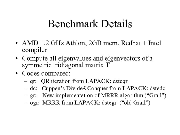
Benchmark Details • AMD 1. 2 GHz Athlon, 2 GB mem, Redhat + Intel compiler • Compute all eigenvalues and eigenvectors of a symmetric tridiagonal matrix T • Codes compared: – – qr: QR iteration from LAPACK: dsteqr dc: Cuppen’s Divide&Conquer from LAPACK: dstedc gr: New implementation of MRRR algorithm (“Grail”) ogr: MRRR from LAPACK: dstegr (“old Grail”)
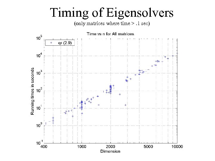
Timing of Eigensolvers (only matrices where time >. 1 sec)
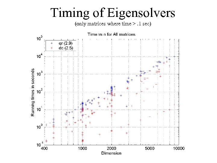
Timing of Eigensolvers (only matrices where time >. 1 sec)
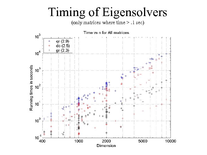
Timing of Eigensolvers (only matrices where time >. 1 sec)
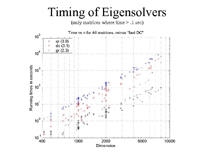
Timing of Eigensolvers (only matrices where time >. 1 sec)
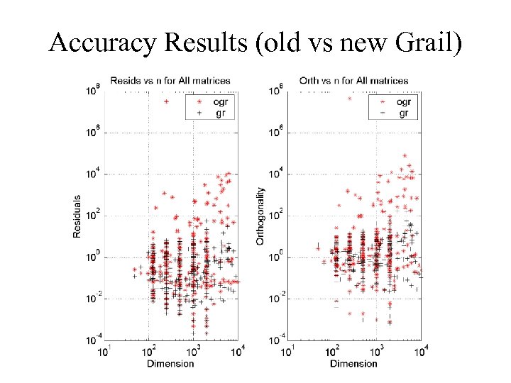
Accuracy Results (old vs new Grail)
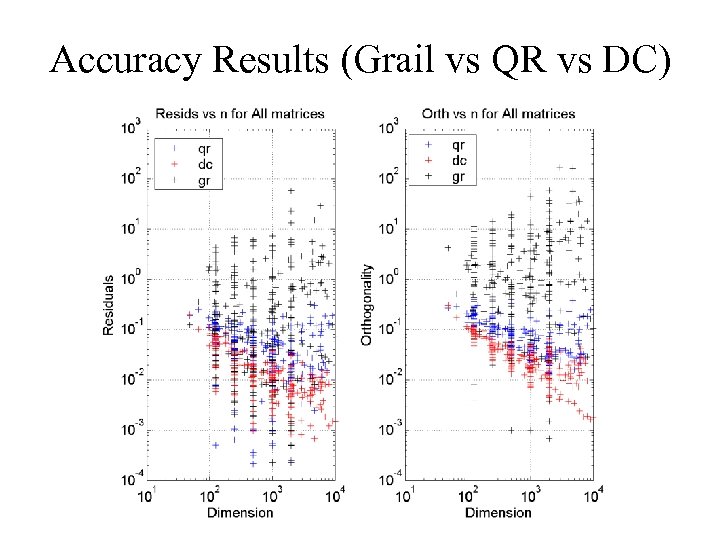
Accuracy Results (Grail vs QR vs DC)
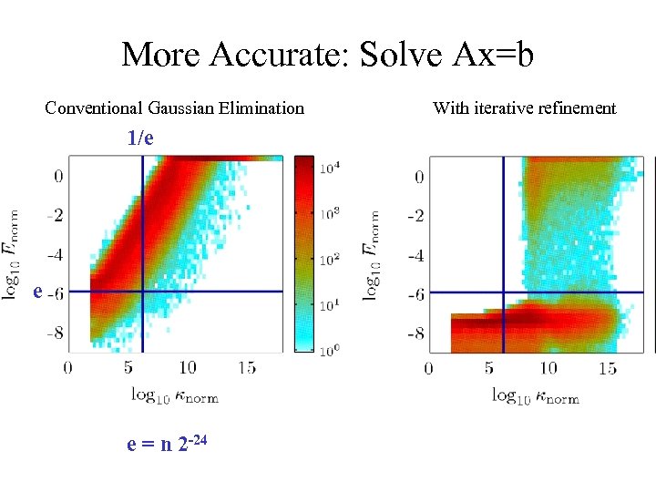
More Accurate: Solve Ax=b Conventional Gaussian Elimination 1/e e e = n 2 -24 With iterative refinement
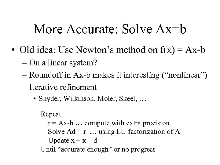
More Accurate: Solve Ax=b • Old idea: Use Newton’s method on f(x) = Ax-b – On a linear system? – Roundoff in Ax-b makes it interesting (“nonlinear”) – Iterative refinement • Snyder, Wilkinson, Moler, Skeel, … Repeat r = Ax-b … compute with extra precision Solve Ad = r … using LU factorization of A Update x = x – d Until “accurate enough” or no progress
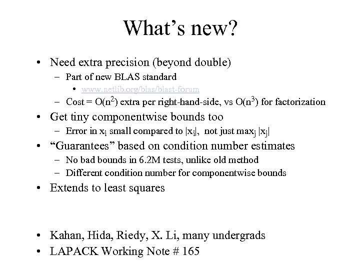
What’s new? • Need extra precision (beyond double) – Part of new BLAS standard • www. netlib. org/blast-forum – Cost = O(n 2) extra per right-hand-side, vs O(n 3) for factorization • Get tiny componentwise bounds too – Error in xi small compared to |xi|, not just maxj |xj| • “Guarantees” based on condition number estimates – No bad bounds in 6. 2 M tests, unlike old method – Different condition number for componentwise bounds • Extends to least squares • Kahan, Hida, Riedy, X. Li, many undergrads • LAPACK Working Note # 165
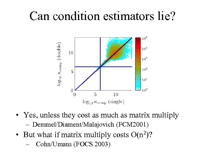
Can condition estimators lie? • Yes, unless they cost as much as matrix multiply – Demmel/Diament/Malajovich (FCM 2001) • But what if matrix multiply costs O(n 2)? – Cohn/Umans (FOCS 2003)
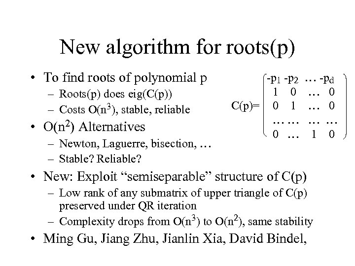
New algorithm for roots(p) • To find roots of polynomial p – Roots(p) does eig(C(p)) – Costs O(n 3), stable, reliable • O(n 2) Alternatives – Newton, Laguerre, bisection, … – Stable? Reliable? -p 1 -p 2 1 0 C(p)= 0 1 …… 0 … … -pd … 0 … … 1 0 • New: Exploit “semiseparable” structure of C(p) – Low rank of any submatrix of upper triangle of C(p) preserved under QR iteration – Complexity drops from O(n 3) to O(n 2), same stability • Ming Gu, Jiang Zhu, Jianlin Xia, David Bindel,
Conclusions • Lots of opportunities for faster and more accurate solutions to classical problems • Tuning algorithms for problems and architectures – Automated search to deal with complexity – Surprising optima, “needle in a haystack” • Exploiting mathematical structure to find faster algorithms
Thanks to NSF and DOE for support These slides available at www. cs. berkeley. edu/~demmel/Utah_Apr 05. ppt
8c637ad4c55fce4d499fde1a01967cc2.ppt