The Economics of Climate Change The basic

The Economics of Climate Change

The basic mechanism

In the long run perspective

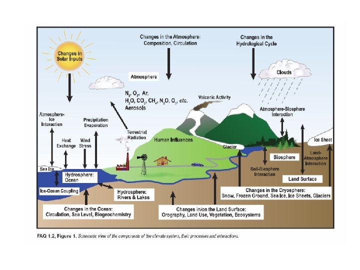
Do not mix up with Ozone layers • Both are environmental problems • Both are related to the atmosphere • But they different issues – The atomosphere is so complex that more than one process may go on there • The ozone layer stop ultra-violet rays – With a thin ozone layer, skin cancer more likely – But note: This is an example demonstrating that international agreement can be successful! • Global warming is an other problem

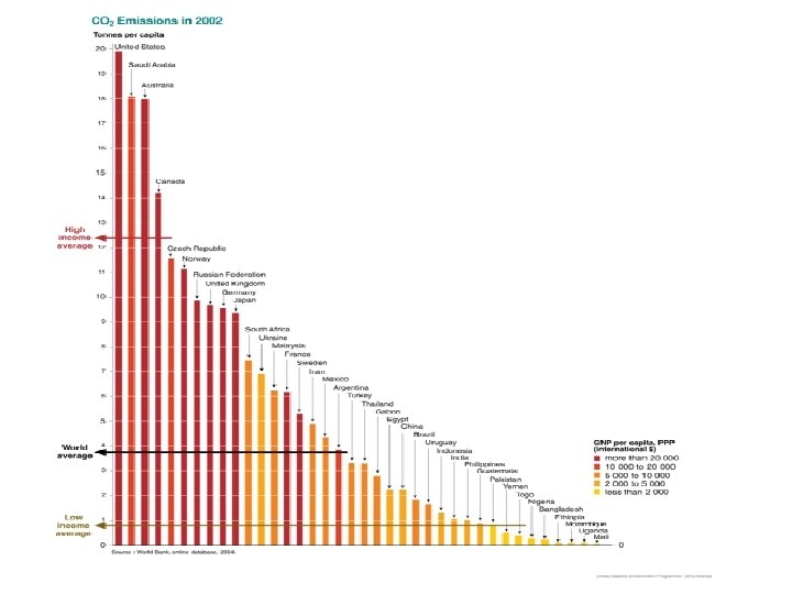
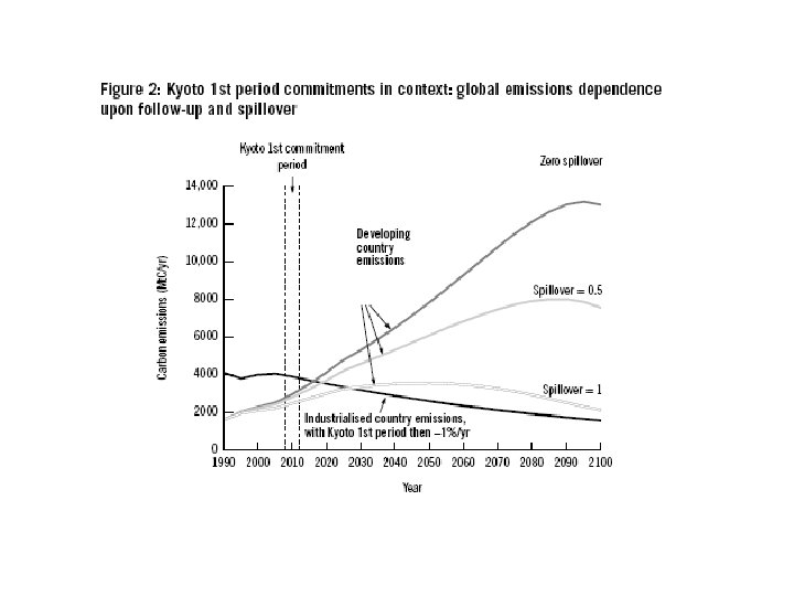
International agreement • The problems of reaching an agreement on CO 2 is eminent. • In addition to the incentives discussed, we have distributional issues. – The cost likely to be born by developing countries – These countries have not caused the problems. – Equal emission cut in % will harm the poor – Equal emissions per capita will gain China and India hugely.

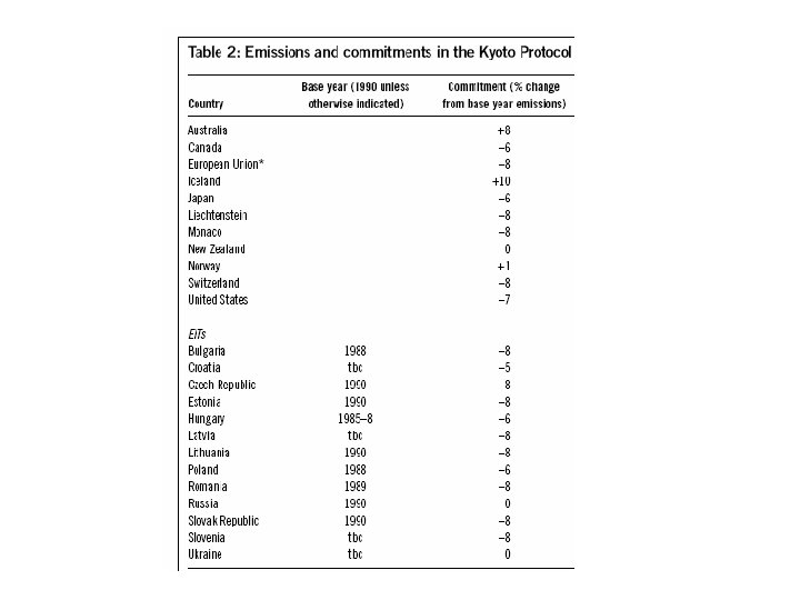
The Kyoto protocol • Agreement from December 1997 • Annex I: Countries listed to take cut in emission – Countries with emissions above 2 t. C/cap 1990 • Reductions relative to 1990 -level. – Not by populations or GDP – Avoid strategic emissions • Annex I countries may induce reduction in Non -Annex I countries through Clean Development mechanisms (CDM)

Emissions 2000 relative to target

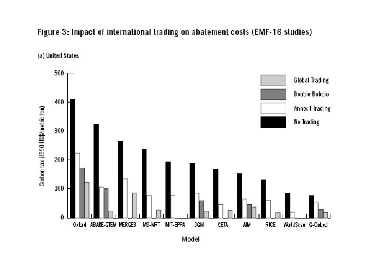
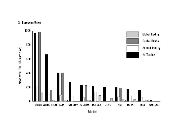
Emission trading in Kyoto • Was controversial in negotiations – Concern about market power from large sellers (Russia) and buyers (US) – Resistance to emission trading in general. • Two main mechanism – Clean Development Mechanism (CDM) Countries with comittments can pay for development projects in countries without committment provided these would not be undertaken otherwise. – Joint implementation: Two or more countries with committment can jointly implement their committment (Trade quotas; EU has redistributed their quota and established a market)

Returning to optimal policy Recall from last week • Nordhaus find an optimal carbon price of 27$/t. C • Stern find an optimal carbon price at 250$/t. C • The main different is the discount rate – The Stern review implicitly uses 1. 4% – Nordhaus uses 4% discount rate, but a 6% return on capital.

Return to investments • If we invest 1 million $ today, what will it be worth 100 years from now: – In Treasury Bills: at most 2, 7 million $ (1%) – In stocks: 2, 2 billion $ (historical return, 8%) • Why this huge difference? – Uncertainty explains some of the difference – But not all of it – Returns to stock may be lower if we estimate it today.

A Crash-course in Finance; CAPM • An investor is better of owning 50% of two firms than 100% of one. – If one firm get bankrupt he is still not broke. • The best hedged portfolio owns a share of all stocks. (The market portfolio) • Now consider selling 1000 $ of the portfolio and buy stock A: Will the portfolio be more or less risky? – Depends on the correlation with the market portfolio.

Example: To assets • Both A and B pays 1 million Kroner with probability 0. 1%, otherwise nothing? – Are they equally risky? • Depends on how they correlate with your wealth: – A pay 1 million if your house burns. – B pay 1 million if the stock market is excep. good. • A makes you wealth less uncertain, B makes it more uncertain.

The Capital Asset Pricing Model (CAPM)

Does climate abatement add to future uncertainty? • Nordhaus: D’(A) is positively correlated with future GDP. – There is more at stake when future GDP is high – Implies a discount rate above the Treasury bill (1%) • Howarth estimate the CAPM model and finds a discount rate much closer to 1% than to 8%.

Temperature change and consumption

Subjective probabilities and tails • Difficult to estimate probabilities – Not like a dice we can roll hundreds of times and observe frequencies • The rare events that we almost never observe, may be the most important.

The equity premium puzzle • If stock pay 7% more than bonds, why don’t we put all our wealth into bonds? – Risk aversion must be implausibly high to explain it – The returns to stock may be overestimated? – Some other theories, resolution of uncertainty, behavioral economics, etc. • The implication for climate discounting not well studied.

The tick tail (Weitzman) • Consider the St. Petersburg paradox – Flip a coin until tail in n’th flip – Payment 2 to the n’th, 2, 4, 8, 16, 32… – Expected value • If we run 100 000 simulation, we will most likely not observe n above 30 – Estimated value will be rather small • With 100 000 observation we will miss the tail – And hence miss the real expected value • In climate chance the extreme event are important, events we do not observe and no model simulates

Assessing the tail of climate change (Weitzman) • There are hundreds of simulation of temperature change provided we stabilize at 560 ppm (2 x 280 ppm, the preindustrial level) • 1% of these give temperature change > 10 degree – The premise ignores feedback, methane will be released from the tundra, likely temperature increase is up to 20 degrees; the difference between summer and winter in Oslo. – No guarantee that mankind will survive – D’(A) and GDP negatively correlated – Weitzman conclude that the optimal carbon price is almost infinite. • Note: It is highly unlikely that the world will be able to stabilize CO 2 at a level as low as 560 ppm